Moving mass at least cost: the Monge and Kantorovich problems of optimal transport
Given two probability distributions and a cost for moving a unit of mass from one point to another, optimal transport asks for the cheapest way to rearrange the first distribution into the second. The question was posed by Monge in 1781 for piles of earth and was reformulated by Kantorovich in 1942 in a form that turned out to be a linear program. The resulting distances between distributions, the Wasserstein distances, are now used throughout probability and statistics. Below, Kantorovich’s relaxation is motivated and shown to always have a solution, and the solution is described in three cases: discrete measures, measures on the line, and quadratic cost in \(\R^d\). The last section treats entropic regularization, which makes the discrete problem fast to solve.
Throughout, \(\mathcal X\) and \(\mathcal Y\) are Polish spaces (complete separable metric spaces), \(\mu\) and \(\nu\) are Borel probability measures on them, and \(c : \mathcal X \times \mathcal Y \to [0, \infty]\) is a lower semicontinuous cost. For a Borel map \(T\), the push-forward \(T_\#\mu\) is the measure \(B \mapsto \mu(T^{-1}(B))\).
Monge’s problem and why it needs relaxing
Monge’s problem is to minimize
\[\int_{\mathcal X} c\bigl(x, T(x)\bigr)\, \mu(\dd x) \quad \text{over Borel maps } T : \mathcal X \to \mathcal Y \text{ with } T_\#\mu = \nu .\]Three features make it hard to treat directly. The set of admissible maps can be empty: if \(\mu = \delta_0\) and \(\nu = \tfrac12(\delta_{-1} + \delta_1)\), every push-forward of \(\mu\) is a point mass, so no map works; mass at a point cannot be split. The constraint \(T_\#\mu = \nu\) is nonlinear in \(T\) and is not preserved under the weak limits that compactness arguments produce. And the infimum need not be attained even when admissible maps exist. In \(\R^2\) with \(c(x, y) = \norm{x - y}\), let \(\mu\) be uniform on the segment \(\{0\} \times [0, 1]\) and \(\nu\) put mass \(\tfrac12\) uniformly on each of \(\{-1\} \times [0, 1]\) and \(\{1\} \times [0,1]\). Every point moves at least distance \(1\), so every admissible map costs at least \(1\). Cutting \([0,1]\) into \(k\) intervals, sending the lower half of each to the left segment and the upper half to the right one, each stretched by a factor \(2\) over the whole interval, gives an admissible map with vertical displacements at most \(1/k\) and cost at most \(\sqrt{1 + k^{-2}}\). So the infimum is \(1\). A map with cost exactly \(1\) would have to move every point horizontally, \(T(0, t) = (\pm 1, t)\), and then the image of the set of \(t\) sent to the right would carry density \(1\) on that set, never the required density \(\tfrac12\).
Kantorovich’s relaxation
A coupling of \(\mu\) and \(\nu\) is a probability measure \(\pi\) on \(\mathcal X \times \mathcal Y\) with marginals \(\mu\) and \(\nu\); write \(\Pi(\mu, \nu)\) for the set of couplings. Kantorovich’s problem is
\[K(\mu, \nu) = \inf_{\pi \in \Pi(\mu, \nu)} \int c \,\dd\pi .\]The value \(\pi(A \times B)\) is the amount of mass moved from \(A\) to \(B\), and mass at a point may now be split. The set \(\Pi(\mu, \nu)\) is convex and never empty, since it contains \(\mu \otimes \nu\), and the objective is linear in \(\pi\). Every admissible map \(T\) yields the coupling \((\mathrm{id}, T)_\#\mu\) with the same cost, so \(K(\mu, \nu)\) is at most the Monge infimum. In the two-segment example the coupling that sends half of each point’s mass to each side costs exactly \(1\).
Theorem 1. Under the standing assumptions (\(\mathcal X, \mathcal Y\) Polish, \(c \ge 0\) lower semicontinuous), there is \(\pi^* \in \Pi(\mu, \nu)\) with \(\int c\,\dd\pi^* = K(\mu, \nu)\).
Proof. Compactness. On a Polish space every Borel probability measure is tight, so for \(\varepsilon > 0\) there are compact sets \(K_1 \subseteq \mathcal X\), \(K_2 \subseteq \mathcal Y\) with \(\mu(K_1^c) < \varepsilon\) and \(\nu(K_2^c) < \varepsilon\). For every \(\pi \in \Pi(\mu, \nu)\),
\[\pi\bigl((K_1 \times K_2)^c\bigr) \le \pi(K_1^c \times \mathcal Y) + \pi(\mathcal X \times K_2^c) < 2\varepsilon ,\]so \(\Pi(\mu, \nu)\) is tight and, by Prokhorov’s theorem, relatively compact for weak convergence. It is also closed: the coordinate projections are continuous, so if \(\pi_k \Rightarrow \pi\) then the marginals of \(\pi_k\) converge weakly to those of \(\pi\), which are therefore \(\mu\) and \(\nu\).
Lower semicontinuity. Fix a metric \(d\) on \(\mathcal X \times \mathcal Y\) compatible with its topology and set
\[c_k(z) = \inf_{w}\bigl\{\min\{c(w), k\} + k\, d(z, w)\bigr\}, \qquad k \in \N .\]Each \(c_k\) is \(k\)-Lipschitz (an infimum of \(k\)-Lipschitz functions), satisfies \(0 \le c_k \le \min\{c, k\}\) (take \(w = z\)), and \(c_k \le c_{k+1}\). Moreover \(c_k(z) \to c(z)\): otherwise there are \(L < c(z)\) and, for each \(k > L\), a point \(w_k\) with \(\min\{c(w_k), k\} + k\,d(z, w_k) < L\); then \(d(z, w_k) < L/k \to 0\) and \(c(w_k) < L\), contradicting \(\liminf_k c(w_k) \ge c(z)\). By monotone convergence \(\int c\,\dd\pi = \sup_k \int c_k\,\dd\pi\), a supremum of weakly continuous functions of \(\pi\), hence weakly lower semicontinuous.
Conclusion. Take \(\pi_k \in \Pi(\mu, \nu)\) with \(\int c\,\dd\pi_k \to K(\mu, \nu)\). A subsequence converges weakly to some \(\pi^* \in \Pi(\mu, \nu)\), and lower semicontinuity gives \(\int c\,\dd\pi^* \le K(\mu, \nu)\).
For \(p \ge 1\) and measures on a metric space with finite \(p\)th moments, \(W_p(\mu, \nu) = K(\mu, \nu)^{1/p}\) with \(c = d^p\) is the \(p\)-Wasserstein distance; it is a metric, and it metrizes weak convergence together with convergence of \(p\)th moments.
Discrete measures: a linear program
Let \(\mu = \sum_{i=1}^m a_i \delta_{x_i}\) and \(\nu = \sum_{j=1}^n b_j \delta_{y_j}\) with positive weights, and \(C_{ij} = c(x_i, y_j)\). A coupling is a matrix in the transportation polytope \(U(a, b) = \{P \in \R^{m \times n} : P \ge 0,\ P\mathbf 1_n = a,\ P^\top \mathbf 1_m = b\}\), and the problem is the linear program of minimizing \(\inner{C}{P} = \sum_{ij} C_{ij}P_{ij}\) over \(U(a, b)\). Its dual is
\[\max_{f \in \R^m,\, g \in \R^n} \ \sum_i a_i f_i + \sum_j b_j g_j \quad \text{subject to } f_i + g_j \le C_{ij} \text{ for all } i, j .\]Both problems are feasible, so by linear programming duality their optimal values coincide, and complementary slackness says that an optimal \(P\) moves mass from \(x_i\) to \(y_j\) only when \(f_i + g_j = C_{ij}\). The dual variables can be read as prices, \(-f_i\) paid for a unit of mass at \(x_i\) and \(g_j\) received for it at \(y_j\); the constraint says that no such price difference exceeds the cost of transport. Since \(U(a, b)\) is a compact polytope, the minimum is attained at a vertex. The \(m + n\) equality constraints have rank \(m + n - 1\) (both families sum to \(1\)), so a vertex has at most \(m + n - 1\) nonzero entries: optimal plans can be chosen sparse, splitting the mass of only a few points.
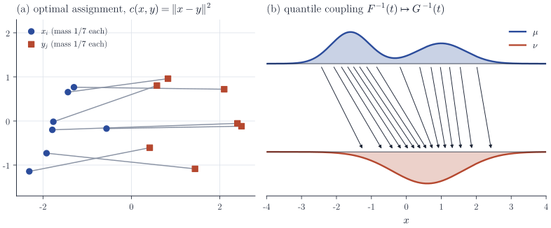
When \(m = n\) and \(a_i = b_j = 1/n\), \(U(a, b)\) is \(1/n\) times the set of doubly stochastic matrices, whose extreme points are the permutation matrices by the Birkhoff–von Neumann theorem. Hence some optimal coupling is induced by a permutation: the relaxation has a Monge solution, and the problem is the assignment problem. Figure 1(a) shows an example solved by enumerating all \(7! = 5040\) permutations.
Measures on the line
On \(\R\) the solution is explicit for costs \(c(x, y) = h(x - y)\) with \(h\) convex. The mechanism is visible already for \(n\) points of equal mass.
Proposition 2. Let \(h : \R \to [0, \infty)\) be convex, \(x_1 \le \cdots \le x_n\) and \(y_1 \le \cdots \le y_n\). Among all permutations \(\sigma\), the sum \(\sum_i h(x_i - y_{\sigma(i)})\) is minimized by the identity.
Proof. If \(p \le s, t \le q\) and \(s + t = p + q\), then \(s = \lambda p + (1 - \lambda) q\) and \(t = (1-\lambda)p + \lambda q\) for some \(\lambda \in [0,1]\), and convexity gives \(h(s) + h(t) \le h(p) + h(q)\). Suppose \(i < j\) but \(\sigma(i) > \sigma(j)\), and put \(y = y_{\sigma(j)} \le y' = y_{\sigma(i)}\). The four numbers \(p = x_i - y'\), \(q = x_j - y\), \(s = x_i - y\), \(t = x_j - y'\) satisfy \(p \le s, t \le q\) and \(s + t = p + q\), so exchanging the targets of \(i\) and \(j\) does not increase the cost. Each exchange removes at least one inversion of \(\sigma\), so finitely many exchanges reach the identity.
For general measures, let \(F\) and \(G\) be the distribution functions of \(\mu\) and \(\nu\) and \(F^{-1}(t) = \inf\{x : F(x) \ge t\}\) the quantile function. The monotone (comonotone) coupling is the law of \((F^{-1}(V), G^{-1}(V))\) with \(V\) uniform on \((0,1)\), the continuous analogue of matching the \(k\)th smallest point with the \(k\)th smallest point.
Theorem 3. Let \(h : \R \to [0, \infty)\) be convex and \(c(x, y) = h(x - y)\). For all Borel probability measures \(\mu, \nu\) on \(\R\), the monotone coupling is optimal, so
\[K(\mu, \nu) = \int_0^1 h\bigl(F^{-1}(t) - G^{-1}(t)\bigr)\, \dd t .\]If \(\mu\) has no atoms, the map \(T = G^{-1} \circ F\) satisfies \(T_\#\mu = \nu\) and is an optimal Monge map.
One route to the general statement approximates \(\mu\) and \(\nu\) by measures with \(n\) equal atoms at their quantiles, applies Proposition 2, and passes to the limit using the stability of optimal couplings under weak convergence; complete proofs are in Chapter 2 of Santambrogio’s book. The last claim is elementary: if \(F\) is continuous then \(F(X)\) is uniform on \((0,1)\) for \(X \sim \mu\), so \(G^{-1}(F(X)) \sim \nu\) by the inverse-transform method, and the coupling \((X, T(X))\) is the monotone one because \(F^{-1}(F(X)) = X\) almost surely. In particular \(W_p^p(\mu, \nu) = \int_0^1 \abs{F^{-1}(t) - G^{-1}(t)}^p\,\dd t\), and for \(p = 1\) the integral of \(\abs{F^{-1} - G^{-1}}\) over \((0,1)\) and the integral of \(\abs{F - G}\) over \(\R\) both compute the area between the graphs of \(F\) and \(G\), so \(W_1(\mu, \nu) = \int_{\R} \abs{F(x) - G(x)}\,\dd x\).
Quadratic cost in several dimensions
In \(\R^d\) with \(c(x, y) = \norm{x - y}^2\) the monotone map has a multivariate counterpart.
Theorem 4 (Brenier). Let \(\mu, \nu\) be probability measures on \(\R^d\) with finite second moments, and assume \(\mu\) is absolutely continuous with respect to Lebesgue measure. Then there is exactly one optimal coupling for the cost \(\norm{x - y}^2\). It has the form \((\mathrm{id}, \nabla\varphi)_\#\mu\) for a convex function \(\varphi : \R^d \to \R \cup \{+\infty\}\) that is differentiable \(\mu\)-almost everywhere, and \(\nabla\varphi\) is uniquely determined \(\mu\)-almost everywhere.
Here is the structure of the proof; details are in Brenier (1991) and in Chapter 2 of Villani’s Topics in Optimal Transportation. Expanding \(\norm{x - y}^2 = \norm x^2 + \norm y^2 - 2\inner{x}{y}\), finite second moments make the first two terms constant over \(\Pi(\mu, \nu)\), so optimal couplings are exactly those maximizing \(\int \inner{x}{y}\,\dd\pi\). Kantorovich duality for this problem produces a proper lower semicontinuous convex \(\varphi\) and its convex conjugate \(\varphi^*\) such that \(\varphi(x) + \varphi^*(y) \ge \inner{x}{y}\) for all \(x, y\), with equality \(\pi\)-almost everywhere for every optimal coupling \(\pi\). Equality in this Fenchel–Young inequality means \(y \in \partial\varphi(x)\), the subdifferential; in particular \(\varphi(x) < \infty\) for \(\mu\)-almost every \(x\). A convex function is locally Lipschitz in the interior of its domain, hence differentiable Lebesgue-almost everywhere there, and the boundary of a convex set is Lebesgue-null. Since \(\mu\) has a density, \(\partial\varphi(x) = \{\nabla\varphi(x)\}\) for \(\mu\)-almost every \(x\), and every optimal coupling is concentrated on the graph of \(\nabla\varphi\). A coupling with first marginal \(\mu\) that is concentrated on the graph of a map \(T\) equals \((\mathrm{id}, T)_\#\mu\); since the same \(\varphi\) serves for every optimal coupling, all of them equal \((\mathrm{id}, \nabla\varphi)_\#\mu\), which proves uniqueness. McCann (1995) showed, without moment assumptions, that the gradient of a convex function pushing \(\mu\) to \(\nu\) is unique \(\mu\)-almost everywhere. In one dimension \(\nabla\varphi = \varphi'\) is nondecreasing, and Theorem 4 reduces to Theorem 3.
Gaussian measures give a closed form. Let \(\mu = \mathcal N(m_1, \Sigma_1)\) with \(\Sigma_1\) positive definite and \(\nu = \mathcal N(m_2, \Sigma_2)\), and set
\[A = \Sigma_1^{-1/2}\bigl(\Sigma_1^{1/2}\Sigma_2\Sigma_1^{1/2}\bigr)^{1/2}\Sigma_1^{-1/2}, \qquad T(x) = m_2 + A(x - m_1).\]The matrix \(A\) is symmetric positive semidefinite, so \(T\) is the gradient of the convex function \(\varphi(x) = \inner{m_2}{x} + \tfrac12 (x - m_1)^\top A (x - m_1)\). Writing \(M = (\Sigma_1^{1/2}\Sigma_2\Sigma_1^{1/2})^{1/2}\), one checks \(A\Sigma_1 A = \Sigma_1^{-1/2} M^2 \Sigma_1^{-1/2} = \Sigma_2\), so \(T_\#\mu = \nu\). Optimality follows from the Fenchel–Young inequality: for any coupling \(\pi\) of \(\mu\) and \(\nu\), \(\int \inner{x}{y}\,\dd\pi \le \int\varphi\,\dd\mu + \int\varphi^*\,\dd\nu\), with equality for \((\mathrm{id}, \nabla\varphi)_\#\mu\) because \(\varphi(x) + \varphi^*(\nabla\varphi(x)) = \inner{x}{\nabla\varphi(x)}\). Here \(\varphi\) is a quadratic polynomial and \(\varphi^*\) is a quadratic polynomial on the affine subspace \(m_2 + \operatorname{range}(\Sigma_2)\) that carries \(\nu\) (the range of \(A\) is that of \(\Sigma_2\)), so both integrals are finite. The same argument shows that any \(\nabla\varphi\) with \(\varphi\) convex, \((\nabla\varphi)_\#\mu = \nu\), \(\varphi \in L^1(\mu)\) and \(\varphi^* \in L^1(\nu)\) is an optimal map. The cost of \(T\) is
\[W_2^2(\mu, \nu) = \norm{m_1 - m_2}^2 + \tr\Sigma_1 + \tr\Sigma_2 - 2\tr\bigl(\Sigma_1^{1/2}\Sigma_2\Sigma_1^{1/2}\bigr)^{1/2},\]using \(\E\norm{(I - A)(X - m_1)}^2 = \tr\Sigma_1 - 2\tr(A\Sigma_1) + \tr(A\Sigma_1A)\) and \(\tr(A\Sigma_1) = \tr(\Sigma_1^{-1/2} M \Sigma_1^{1/2}) = \tr M\).
Entropic regularization and Sinkhorn’s algorithm
General linear programming solvers for discrete transport scale poorly with \(m\) and \(n\). Adding an entropy term changes the problem into one with a closed-form structure. For \(\varepsilon > 0\) consider
\[\min_{P \in U(a,b)}\ \inner{C}{P} + \varepsilon \sum_{i,j} P_{ij}\bigl(\log P_{ij} - 1\bigr), \qquad 0 \log 0 = 0 .\]Proposition 5. For every \(\varepsilon > 0\) the regularized problem has a unique solution \(P^\varepsilon\). Its entries are positive and it has the form
\[P^\varepsilon_{ij} = u_i\, e^{-C_{ij}/\varepsilon}\, v_j\]for positive vectors \(u \in \R^m\), \(v \in \R^n\).
Proof. The objective is continuous and strictly convex on the compact convex set \(U(a,b)\), so the minimizer exists and is unique. Suppose \(P^\varepsilon_{ij} = 0\) for some \((i, j)\) and let \(P_t = (1-t)P^\varepsilon + t\, ab^\top\), which lies in \(U(a,b)\) and has all entries positive for \(t \in (0, 1]\). The function \(s \mapsto s\log s\) has derivative \(-\infty\) at \(0^+\), while the remaining terms of the objective have finite one-sided derivatives in \(t\) at \(0\); hence the objective along \(P_t\) has derivative \(-\infty\) at \(t = 0^+\) and decreases for small \(t\), a contradiction. So \(P^\varepsilon\) lies in the relative interior of \(U(a,b)\), where only the affine constraints are active, and the Lagrange conditions give multipliers \(f_i, g_j\) with \(C_{ij} + \varepsilon\log P^\varepsilon_{ij} = f_i + g_j\). Set \(u_i = e^{f_i/\varepsilon}\) and \(v_j = e^{g_j/\varepsilon}\).
With \(K_{ij} = e^{-C_{ij}/\varepsilon}\), the marginal constraints become \(u \odot (Kv) = a\) and \(v \odot (K^\top u) = b\). Sinkhorn’s algorithm solves them by alternation,
\[u \leftarrow a \oslash (K v), \qquad v \leftarrow b \oslash (K^\top u),\]each step enforcing one family of marginals exactly. Sinkhorn (1964) proved that a square matrix with positive entries can be scaled in this way to a doubly stochastic matrix, the case \(a = \mathbf 1_n/n\), \(b = \mathbf 1_n/n\) up to normalization; for positive \(K\) and general marginals the iteration converges geometrically, at a rate that deteriorates as \(\varepsilon \to 0\). Each iteration costs two matrix–vector products, which is the reason for its popularity in machine learning since Cuturi (2013). Equivalently, the iteration is block coordinate ascent on the concave dual \(\sum_i a_i f_i + \sum_j b_j g_j - \varepsilon\sum_{ij} e^{(f_i + g_j - C_{ij})/\varepsilon}\). For small \(\varepsilon\) the entries of \(K\) underflow, and the same updates are carried out on \(f\) and \(g\) with log-sum-exp:
import numpy as np
from scipy.special import logsumexp

def sinkhorn_log(a, b, C, eps, iters=2000):
    f, g = np.zeros(len(a)), np.zeros(len(b))
    for _ in range(iters):
        f = eps * np.log(a) - eps * logsumexp((g[None, :] - C) / eps, axis=1)
        g = eps * np.log(b) - eps * logsumexp((f[:, None] - C) / eps, axis=0)
    return np.exp((f[:, None] + g[None, :] - C) / eps)
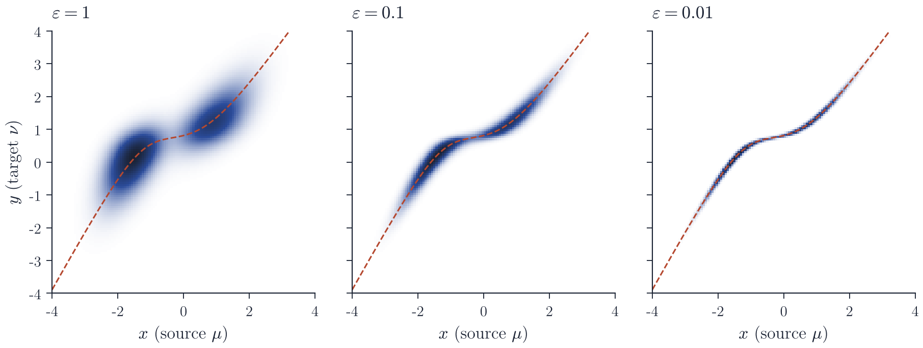
As \(\varepsilon \to \infty\) the plan tends to the independent coupling \(ab^\top\), and as \(\varepsilon \to 0\) it converges to an optimal plan of the linear program. Figure 2 shows this for discretized versions of the two measures of Figure 1(b): the plans concentrate around the graph of the monotone map \(G^{-1} \circ F\) of Theorem 3.
Remarks
Kantorovich duality, used above only in outline, holds in the generality of Theorem 1: \(K(\mu, \nu) = \sup\{\int f\,\dd\mu + \int g\,\dd\nu\}\) over bounded continuous \(f, g\) with \(f(x) + g(y) \le c(x, y)\). Its proof, the characterization of optimal couplings by cyclical monotonicity of their supports, and the metric properties of \(W_p\) are in Villani, Topics in Optimal Transportation (AMS, 2003) and Optimal Transport: Old and New (Springer, 2009), and in Santambrogio, Optimal Transport for Applied Mathematicians (Birkhäuser, 2015). The original sources for the two main results are Brenier, Polar factorization and monotone rearrangement of vector-valued functions (Comm. Pure Appl. Math., 1991), and McCann, Existence and uniqueness of monotone measure-preserving maps (Duke Math. J., 1995). For the computational side, including Sinkhorn’s algorithm and its variants, see Peyré and Cuturi, Computational Optimal Transport (Foundations and Trends in Machine Learning, 2019).