Does the posterior find the truth? Prior mass, tests and Schwartz's theorem
A Bayesian analysis produces a posterior distribution, and one can ask a frequentist question about it. Suppose the data really are independent draws from a fixed distribution \(P_0\). As the sample grows, does the posterior pile up near \(P_0\)? The answer is not automatic. It can fail when the prior ignores the truth, and in infinite-dimensional models it can fail in subtler ways. Two classical results frame the subject: Doob’s theorem, which is general but says little about any particular truth, and Schwartz’s theorem, which isolates the two properties that make consistency work.
Setting
Let \((\mathcal X, \mathcal A)\) be a measurable space with a \(\sigma\)-finite measure \(\mu\), and let \(\mathcal P\) be a set of probability densities with respect to \(\mu\), equipped with a \(\sigma\)-field for which \((x, p) \mapsto p(x)\) is jointly measurable. A prior is a probability measure \(\Pi\) on \(\mathcal P\); parametric models are the special case \(\mathcal P = \{p_\theta : \theta \in \Theta\}\). The observations \(X_1, X_2, \dots\) are independent with density \(p_0\), which need not belong to \(\mathcal P\), and \(P_0^\infty\) denotes their joint law. The posterior after \(n\) observations is
\[\Pi_n(A) = \frac{\int_A \prod_{i=1}^n p(X_i) \, \dd\Pi(p)}{\int_{\mathcal P} \prod_{i=1}^n p(X_i) \, \dd\Pi(p)},\]defined whenever the denominator is positive and finite.
The posterior is (strongly) consistent at \(p_0\) with respect to a topology on \(\mathcal P\) if \(\Pi_n(U^c) \to 0\) \(P_0^\infty\)-almost surely for every neighbourhood \(U\) of \(p_0\). In a parametric model one usually takes \(U = \{p_\theta : \norm{\theta - \theta_0} < \varepsilon\}\).
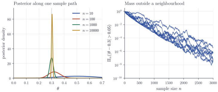
A conjugate example shows what is expected. For Bernoulli data with a \(\mathrm{Beta}(a, b)\) prior the posterior is \(\mathrm{Beta}(a + S_n, b + n - S_n)\), with \(S_n = \sum_{i \le n} X_i\). By the strong law, the posterior mean \((a + S_n)/(a + b + n) \to \theta_0\) almost surely, while the posterior variance is at most \(1/(4(a + b + n + 1))\). Chebyshev’s inequality then gives consistency. Figure 1 shows the posterior narrowing around \(\theta_0\) along one sample path, and shows something sharper: the mass outside a fixed neighbourhood decays exponentially in \(n\). The general argument below explains both.
Doob’s theorem
The first general result needs almost no assumptions, and it is correspondingly weak. Let the sample space \(\mathcal X\) be Polish with its Borel \(\sigma\)-field, let \(\Theta\) be a Borel subset of a Polish space, let \(\theta \mapsto P_\theta\) be measurable and injective, and give \(\theta\) a prior \(\Pi\). Doob’s theorem (1949) states that there is a set \(\Theta_0 \subseteq \Theta\) with \(\Pi(\Theta_0) = 1\) such that the posterior is consistent at every \(\theta \in \Theta_0\).
The idea is short. Under the joint law of \((\theta, X_1, X_2, \dots)\), identifiability together with the strong law for empirical distributions makes \(\theta\) a measurable function of the whole sequence \(X_1, X_2, \dots\); measurability of the inverse is where the Polish assumption enters. For bounded measurable \(f\), Lévy’s upward martingale convergence theorem gives \(\E[f(\theta) \mid X_1, \dots, X_n] \to \E[f(\theta) \mid X_1, X_2, \dots] = f(\theta)\) almost surely under the joint law. Applying this to a countable convergence-determining family of bounded continuous \(f\) gives weak convergence of the posterior to \(\delta_\theta\), and disintegrating the joint law over \(\theta\) turns “almost surely under the joint law” into “for \(\Pi\)-almost every \(\theta\), \(P_\theta^\infty\)-almost surely”.
The weakness is in the exceptional set. It is null under the prior, which is the analyst’s own choice, and nothing prevents it from containing the truth. In a parametric model with a prior that has a positive continuous density this is harmless. In infinite-dimensional models, Freedman (1963) showed for discrete distributions on the integers, and Diaconis and Freedman (1986, Annals of Statistics) showed in a location problem, that the exceptional set can be topologically large and include natural truths. A theorem that applies at a given \(p_0\) is needed.
Schwartz’s theorem
Two quantities control the posterior at \(p_0\). The Kullback–Leibler divergence \(K(p_0, p) = \int p_0 \log(p_0/p) \, \dd\mu\) measures how well a candidate \(p\) explains typical data from \(p_0\); we say that \(p_0\) belongs to the Kullback–Leibler support of \(\Pi\) if
\[\Pi\bigl(p : K(p_0, p) < \varepsilon\bigr) > 0 \qquad \text{for every } \varepsilon > 0 .\]Write the posterior as a ratio with likelihood ratios against \(p_0\):
\[\Pi_n(A) = \frac{N_n(A)}{D_n}, \qquad N_n(A) = \int_A \prod_{i=1}^n \frac{p(X_i)}{p_0(X_i)} \, \dd\Pi(p), \qquad D_n = N_n(\mathcal P).\]The ratio is well defined because \(p_0(X_i) > 0\) almost surely. The first lemma says that Kullback–Leibler support keeps the denominator from collapsing faster than exponentially.
Lemma 1. If \(p_0\) is in the Kullback–Leibler support of \(\Pi\), then for every \(\beta > 0\), \(e^{n\beta} D_n \to \infty\) \(P_0^\infty\)-almost surely.
Proof. Let \(p\) satisfy \(K(p_0, p) < \infty\). The negative part of \(\log(p_0/p)\) is \(P_0\)-integrable, because \(\log u \le u - 1\) gives \(\E_0\bigl[\log(p/p_0)^+\bigr] \le \E_0\bigl[p/p_0\bigr] \le 1\); since \(K(p_0, p) < \infty\), the positive part is integrable as well. By the strong law, \(n^{-1}\sum_{i \le n} \log(p_0/p)(X_i) \to K(p_0, p)\) almost surely.
Let \(\varepsilon = \beta/2\) and \(B = \{p : K(p_0, p) < \varepsilon\}\), so \(\Pi(B) > 0\). The set \(G\) of pairs \((x^\infty, p)\) for which this convergence holds is jointly measurable, and each of its \(p\)-sections with \(p \in B\) has \(P_0^\infty\)-probability one. By Fubini’s theorem, for \(P_0^\infty\)-almost every sequence \(x^\infty\) the set \(\{p \in B : (x^\infty, p) \in G\}\) has \(\Pi\)-measure \(\Pi(B)\). For such a sequence and such \(p\),
\[e^{n\beta} \prod_{i=1}^n \frac{p(x_i)}{p_0(x_i)} = \exp\Bigl\{n\Bigl(\beta - \frac1n \sum_{i=1}^n \log\frac{p_0}{p}(x_i)\Bigr)\Bigr\} \to \infty,\]since the bracket tends to \(\beta - K(p_0, p) > \beta/2\). Fatou’s lemma gives \(\liminf_n e^{n\beta} D_n \ge \int_B \liminf_n e^{n\beta}\prod_i (p/p_0)(x_i) \, \dd\Pi(p) = \infty\).
The numerator is handled by tests. A test is a measurable \(\phi_n = \phi_n(X_1, \dots, X_n)\) with values in \([0, 1]\).
Theorem 2 (Schwartz). Let \(p_0\) be in the Kullback–Leibler support of \(\Pi\), and let \(U\) be a measurable set containing \(p_0\). Suppose there are tests \(\phi_n\) and constants \(C, c > 0\) with
\[\E_{p_0}\phi_n \le C e^{-cn}, \qquad \sup_{p \in \mathcal P \setminus U} \E_p(1 - \phi_n) \le C e^{-cn} \qquad \text{for all } n.\]Then \(\Pi_n(U^c) \to 0\) \(P_0^\infty\)-almost surely, and in fact \(\Pi_n(U^c) \le e^{-cn/4}\) for all large \(n\), almost surely.
Proof. Since \(\Pi_n(U^c) \le 1\),
\[\Pi_n(U^c) \le \phi_n + (1 - \phi_n)\frac{N_n(U^c)}{D_n}.\]The test. By Markov’s inequality, \(P_0(\phi_n > e^{-cn/2}) \le C e^{-cn/2}\), which is summable, so by Borel–Cantelli \(\phi_n \le e^{-cn/2}\) for all large \(n\), almost surely.
The numerator. By Fubini’s theorem, which applies because the integrand is nonnegative and jointly measurable,
\[\E_{p_0}\bigl[(1 - \phi_n)N_n(U^c)\bigr] = \int_{U^c} \E_{p_0}\Bigl[(1 - \phi_n)\prod_{i=1}^n \frac{p(X_i)}{p_0(X_i)}\Bigr] \dd\Pi(p) \le \int_{U^c} \E_p(1 - \phi_n) \, \dd\Pi(p) \le C e^{-cn}.\]The middle inequality is a change of measure, with “\(\le\)” rather than “\(=\)” because \(p\) may put mass where \(p_0\) vanishes. Markov’s inequality and Borel–Cantelli again give \((1 - \phi_n)N_n(U^c) \le e^{-cn/2}\) for all large \(n\), almost surely.
The denominator. By Lemma 1 with \(\beta = c/8\), \(D_n \ge e^{-cn/8}\) for all large \(n\), almost surely. Combining the three bounds, \(\Pi_n(U^c) \le e^{-cn/2} + e^{-cn/2 + cn/8}\), which is at most \(e^{-cn/4}\) once \(n\) is large.
The proof shows how the two conditions divide the work. Kullback–Leibler support guarantees that the data cannot make every candidate look exponentially worse than \(p_0\), so the denominator decays at most at an arbitrarily small exponential rate. The tests guarantee that distant candidates do look exponentially worse, at a fixed rate \(c\). Schwartz (1965, Zeitschrift für Wahrscheinlichkeitstheorie und verwandte Gebiete) assumed only uniformly consistent tests, that is, \(\E_{p_0}\phi_n \to 0\) and \(\sup_{p \notin U}\E_p(1 - \phi_n) \to 0\); for independent observations such tests can always be converted into tests with exponentially small errors of both kinds, by applying a fixed consistent test to blocks of the sample and using Hoeffding’s inequality on the proportion of blocks that reject. The exponential form above is the one used in applications.
Back to the Bernoulli model. For \(\theta_0 \in (0, 1)\) the divergence
\[K(\theta_0, \theta) = \theta_0 \log\frac{\theta_0}{\theta} + (1 - \theta_0)\log\frac{1 - \theta_0}{1 - \theta}\]is continuous in \(\theta\) and vanishes at \(\theta_0\), so \(\theta_0\) is in the Kullback–Leibler support of any prior that gives positive mass to every interval around \(\theta_0\). For \(U = \{\abs{\theta - \theta_0} < \varepsilon\}\) take \(\phi_n = \mathbf 1\{\abs{\bar X_n - \theta_0} \ge \varepsilon/2\}\). Hoeffding’s inequality, \(P_\theta(\abs{\bar X_n - \theta} \ge t) \le 2e^{-2nt^2}\), gives \(\E_{\theta_0}\phi_n \le 2e^{-n\varepsilon^2/2}\); and if \(\abs{\theta - \theta_0} \ge \varepsilon\), then \(\abs{\bar X_n - \theta_0} < \varepsilon/2\) forces \(\abs{\bar X_n - \theta} > \varepsilon/2\), so \(\E_\theta(1 - \phi_n) \le 2e^{-n\varepsilon^2/2}\). Theorem 2 therefore applies to every such prior, conjugate or not, and predicts the exponential decay in Figure 1.
When the prior misses the truth
If the prior gives no mass near \(p_0\), the hypothesis of Lemma 1 fails and the posterior cannot concentrate at \(p_0\). It does not simply wander: it tends to concentrate near the points of the prior’s support that are closest to \(p_0\) in Kullback–Leibler divergence. Figure 2 shows this for the Bernoulli model with \(\theta_0 = 0.3\) and a prior uniform on \([0, 0.2] \cup [0.5, 1]\). The divergence from \(\theta_0\) is \(0.028\) at \(\theta = 0.2\) and \(0.082\) at \(\theta = 0.5\), and the posterior collapses onto the boundary point \(0.2\). The mechanism is visible in the likelihood \(\theta^{S_n}(1-\theta)^{n - S_n}\), which increases on \([0, \bar X_n]\) and decreases on \([\bar X_n, 1]\). Once \(0.2 < \bar X_n < 0.5\), which by the strong law holds for all large \(n\) almost surely, the likelihood on \([0.5, 1]\) is largest at \(0.5\), and the log-likelihood ratio of \(0.5\) against \(0.2\) is \(n\{K(\theta_0, 0.2) - K(\theta_0, 0.5)\} + o(n) = -0.054\,n + o(n)\) almost surely. The far piece of the support is therefore eliminated at an exponential rate, and on \([0, 0.2]\) the increasing likelihood pushes the mass to the endpoint.
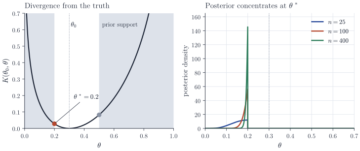
This is the parametric shadow of a general phenomenon. Under misspecification the posterior concentrates near the Kullback–Leibler projection of \(p_0\) onto the support of the prior, under conditions analogous to those of Theorem 2; Kleijn and van der Vaart (2006, Annals of Statistics) develop this in infinite-dimensional models.
Remarks
In parametric models with a smooth prior density, consistency is rarely in doubt, and the Bernstein–von Mises theorem describes the posterior much more precisely. The theory above earns its keep in nonparametric problems. If \(\mathcal P\) carries the weak topology, tests with exponentially small errors exist for every weak neighbourhood, built from averages of bounded continuous functions and Hoeffding’s inequality, so Kullback–Leibler support alone implies weak consistency. For Hellinger or \(L_1\) neighbourhoods, tests exist only if the model is not too large, and the conditions are expressed through metric entropy; see Barron, Schervish and Wasserman (1999, Annals of Statistics) and Ghosal, Ghosh and Ramamoorthi (1999, Annals of Statistics). Rates follow the same pattern with shrinking neighbourhoods: Ghosal, Ghosh and van der Vaart (2000, Annals of Statistics) show that the posterior contracts at rate \(\varepsilon_n\) when the prior puts mass at least \(e^{-Cn\varepsilon_n^2}\) near \(p_0\) and the model can be covered, up to a set of very small prior mass, by about \(e^{cn\varepsilon_n^2}\) balls of radius \(\varepsilon_n\). Ghosal and van der Vaart, Fundamentals of Nonparametric Bayesian Inference, and Ghosh and Ramamoorthi, Bayesian Nonparametrics, give complete treatments.