Power iteration and the eigengap: what sets the rate

The leading eigenvector of a matrix is the direction that the matrix stretches most persistently. Power iteration exploits this literally: multiply a vector by the matrix again and again, normalizing to avoid overflow, and the components along the other eigenvectors shrink relative to the leading one. The method needs only matrix–vector products, so it applies when the matrix is large and available only as an operator, as with a covariance matrix $X^\top X$ that is never formed or the transition matrix of a large graph. Its speed is governed by a single number, the ratio of the two largest eigenvalues in absolute value.

The method

Given $A \in \R^{n \times n}$ and a starting vector $x_0$ with $\lVert x_0\rVert = 1$, iterate

\[x_{k+1} = \frac{A x_k}{\lVert A x_k\rVert}, \qquad \rho_k = x_k^\top A x_k ,\]

where $\rho_k$, the Rayleigh quotient, estimates the eigenvalue. By induction $x_k = A^k x_0 / \lVert A^k x_0\rVert$ as long as no $A^k x_0$ vanishes, so the normalization affects only the scale. In code:

import numpy as np

def power_iteration(matvec, x0, iters):
    x = x0 / np.linalg.norm(x0)
    for _ in range(iters):
        y = matvec(x)
        x = y / np.linalg.norm(y)
    return x, x @ matvec(x)      # eigenvector estimate, Rayleigh quotient

Only matvec touches the matrix. For the leading principal component of a centred $n \times p$ data matrix $X$, matvec = lambda v: X.T @ (X @ v) costs $O(np)$ per iteration, against $O(np^2)$ for forming $X^\top X$.

Convergence for symmetric matrices

Let $A$ be symmetric with eigenvalues ordered by absolute value, $\lvert\lambda_1\rvert > \lvert\lambda_2\rvert \ge \cdots \ge \lvert\lambda_n\rvert$, and orthonormal eigenvectors $v_1, \dots, v_n$. The strict inequality, the eigengap condition, makes the leading eigenvector unique up to sign. Measure the error by the angle $\theta_k \in [0, \pi/2]$ between $x_k$ and the line spanned by $v_1$, so that $\cos\theta_k = \lvert v_1^\top x_k\rvert$; the sign of $x_k$ is irrelevant, and it alternates when $\lambda_1 < 0$.

Theorem 1. If $v_1^\top x_0 \neq 0$, then for every $k \ge 0$

\[\tan\theta_k \le \Bigl\lvert \frac{\lambda_2}{\lambda_1} \Bigr\rvert^{k} \tan\theta_0 , \qquad \lvert \rho_k - \lambda_1\rvert \le 2\lvert\lambda_1\rvert \sin^2\theta_k \le 2\lvert\lambda_1\rvert\, \Bigl\lvert\frac{\lambda_2}{\lambda_1}\Bigr\rvert^{2k} \tan^2\theta_0 .\]

Proof. Expand $x_0 = \sum_j c_j v_j$ with $c_j = v_j^\top x_0$ and $c_1 \neq 0$. Then $A^k x_0 = \sum_j c_j \lambda_j^k v_j$, which is nonzero because its $v_1$-component is $c_1\lambda_1^k \neq 0$ (note $\lambda_1 \neq 0$ by the eigengap condition). Since $x_k$ is a positive multiple of $A^k x_0$ and the $v_j$ are orthonormal,

\[\tan\theta_k = \frac{\bigl(\sum_{j \ge 2} c_j^2\lambda_j^{2k}\bigr)^{1/2}}{\lvert c_1 \lambda_1^k\rvert} \le \Bigl\lvert\frac{\lambda_2}{\lambda_1}\Bigr\rvert^{k}\, \frac{\bigl(\sum_{j\ge 2} c_j^2\bigr)^{1/2}}{\lvert c_1\rvert} = \Bigl\lvert\frac{\lambda_2}{\lambda_1}\Bigr\rvert^{k} \tan\theta_0 ,\]

using $\lvert\lambda_j\rvert \le \lvert\lambda_2\rvert$ for $j \ge 2$.

For the Rayleigh quotient, write the unit vector $x_k = \sum_j a_j v_j$, so that $\sum_j a_j^2 = 1$, $a_1^2 = \cos^2\theta_k$ and $\sum_{j\ge2} a_j^2 = \sin^2\theta_k$. Then

\[\rho_k - \lambda_1 = \sum_j \lambda_j a_j^2 - \lambda_1\sum_j a_j^2 = \sum_{j \ge 2} (\lambda_j - \lambda_1)\, a_j^2 ,\]

and $\lvert\lambda_j - \lambda_1\rvert \le 2\lvert\lambda_1\rvert$. The last inequality uses $\sin\theta \le \tan\theta$ and the first bound.

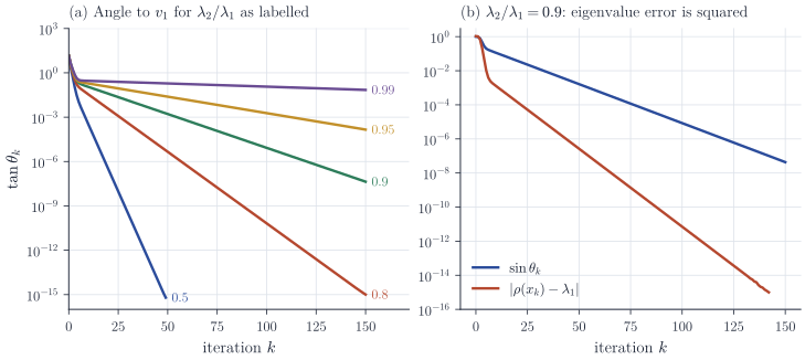
Two features of the theorem deserve comment. First, the rate depends on the ratio $\lvert\lambda_2/\lambda_1\rvert$ and on nothing else about the spectrum: the dimension enters only through the starting angle. To reach $\tan\theta_k \le \varepsilon$ it suffices that

\[k \ge \frac{\log(\tan\theta_0/\varepsilon)}{\log\lvert\lambda_1/\lambda_2\rvert} \approx \frac{1}{\delta}\log\frac{\tan\theta_0}{\varepsilon}, \qquad \delta = 1 - \Bigl\lvert\frac{\lambda_2}{\lambda_1}\Bigr\rvert ,\]

the approximation being accurate for a small relative gap $\delta$. A gap of $1\%$ costs about a hundred iterations per factor of $e$ in accuracy. For a random start, $x_0$ uniform on the sphere, $(v_1^\top x_0)^2$ has a $\mathrm{Beta}(1/2, (n-1)/2)$ distribution with mean $1/n$, so $\tan^2\theta_0$ is typically of order $n$ and contributes only a $\log n$ term.

Second, the eigenvalue converges twice as fast as the eigenvector. The Rayleigh quotient is stationary at eigenvectors (its gradient $2(Ax - \rho(x)x)/\lVert x\rVert^2$ vanishes there), so a first-order error in the vector produces only a second-order error in the value. Figure 1 shows both effects on $200 \times 200$ matrices.

Angle error of power iteration against iteration number for five eigenvalue ratios, and eigenvector versus eigenvalue error for one ratio — Figure 1. Symmetric matrices $A = V\,\mathrm{diag}(\lambda)V^\top$ of size 200 with $\lambda_1 = 1$, $\lambda_2 = r$ and the remaining eigenvalues uniform on $[-r/2, r/2]$; one random orthogonal $V$ and one random start for all runs. (a) After a short transient, during which the components along $v_3, \dots, v_n$ die out, $\tan\theta_k$ decreases geometrically with ratio $r$, as Theorem 1 predicts; curves stop once they reach $10^{-15}$, near rounding level. (b) For $r = 0.9$ the Rayleigh quotient error decreases at rate $r^2$ per iteration, twice the slope of $\sin\theta_k$ on the log scale.

When it fails

The hypotheses of Theorem 1 are both needed.

If $v_1^\top x_0 = 0$, the iterates stay in $v_1^\perp$ in exact arithmetic and converge, under the corresponding gap condition, to the dominant eigenvector of $A$ restricted to that subspace. In floating point, rounding errors reintroduce a small $v_1$-component that then grows, so the failure is a delay. A random starting vector satisfies $v_1^\top x_0 \neq 0$ with probability one.

If there is no gap, $\lvert\lambda_1\rvert = \lvert\lambda_2\rvert$, the method need not converge at all. For $\lambda_2 = \lambda_1$ (and $\lvert\lambda_3\rvert < \lvert\lambda_1\rvert$) the iterates converge to the normalized projection of $x_0$ onto the eigenspace, which is still an eigenvector, but one that depends on the start. For $\lambda_2 = -\lambda_1$ (again with $\lvert\lambda_3\rvert < \lvert\lambda_1\rvert$) the components along $v_1$ and $v_2$ keep the same magnitude and the iterates alternate between two directions forever; the Rayleigh quotient converges to $\lambda_1 (c_1^2 - c_2^2)/(c_1^2 + c_2^2)$, with $c_j = v_j^\top x_0$, which differs from $\pm\lambda_1$ unless $c_1$ or $c_2$ vanishes. The same oscillation occurs for real nonsymmetric matrices whose dominant eigenvalues are a complex conjugate pair.

For nonsymmetric but diagonalizable $A = W\Lambda W^{-1}$, the expansion in the proof still works with the columns of $W$, which are no longer orthogonal. The direction of $x_k$ still converges at rate $\lvert\lambda_2/\lambda_1\rvert^k$, now with a constant depending on the condition number of $W$, while the Rayleigh quotient loses its stationarity and converges only at the same rate as the vector.

Doing better

Since only the ratio matters, any transformation that preserves eigenvectors and improves the ratio helps.

Shifts. The matrix $A - \sigma I$ has the same eigenvectors and eigenvalues $\lambda_j - \sigma$. For a positive semi-definite $A$ with spectrum $\lambda_1 > \lambda_2 \ge \cdots \ge \lambda_n \ge 0$, the shift $\sigma = (\lambda_2 + \lambda_n)/2$ minimizes the dominance ratio, which becomes $(\lambda_2 - \lambda_n)/(2\lambda_1 - \lambda_2 - \lambda_n)$. The gain is modest when $\lambda_n$ is close to zero, and the shift requires knowledge of the spectrum.

Inverse iteration. Power iteration applied to $(A - \sigma I)^{-1}$ converges to the eigenvector whose eigenvalue is closest to $\sigma$, with ratio $\lvert\lambda_{\text{near}} - \sigma\rvert / \lvert\lambda_{\text{next}} - \sigma\rvert$, which is tiny when $\sigma$ is a good eigenvalue estimate. Each step solves a linear system, ideally with a factorization computed once. Updating $\sigma$ to the current Rayleigh quotient at every step gives Rayleigh quotient iteration, which for symmetric matrices converges locally cubically (Parlett, The Symmetric Eigenvalue Problem).

Deflation and subspaces. Once $(\lambda_1, v_1)$ is known for symmetric $A$, power iteration on $A - \lambda_1 v_1v_1^\top$ finds $(\lambda_2, v_2)$, but errors in $v_1$ propagate. It is usually better to iterate a block of $q$ vectors at once and re-orthonormalize with a QR factorization after each multiplication. This subspace (or orthogonal) iteration converges to the span of the top $q$ eigenvectors at rate $\lvert\lambda_{q+1}/\lambda_q\rvert$, so a block slightly larger than the number of eigenvectors wanted can turn a small gap into a large one. Randomized SVD algorithms are subspace iteration with a random start and a few steps.

Krylov methods. Power iteration keeps only the last vector $A^k x_0$ and discards $x_0, Ax_0, \dots, A^{k-1}x_0$. The Lanczos method extracts the best approximation from their span, the Krylov subspace, and for symmetric matrices its convergence is governed by Chebyshev polynomials, with an iteration count that scales roughly like $\delta^{-1/2}$ rather than $\delta^{-1}$ for a small relative gap $\delta$. Library routines for a few eigenvalues of large sparse matrices are Lanczos or Arnoldi methods.

Remarks

Power iteration is rarely the fastest method, but its analysis explains why all the others work and how they can fail: every one of them is limited by gaps in the spectrum, and every one becomes fragile when the eigenvalue of interest is not separated from the rest. In statistics, the eigengap $\lambda_1 - \lambda_2$ also controls how well the leading principal component is determined by a sample covariance matrix, through perturbation bounds of Davis–Kahan type in which it appears in the denominator. Golub and Van Loan, Matrix Computations, treat power, inverse and subspace iteration and the Lanczos method in detail.