Probabilistic PCA from first principles: marginal likelihood, latent posterior and the closed-form maximum
Principal component analysis is defined geometrically, as projection onto the directions of largest variance, and comes with no likelihood. Probabilistic PCA, introduced by Tipping and Bishop (“Probabilistic principal component analysis”, Journal of the Royal Statistical Society, Series B, 1999) and independently by Roweis, supplies one: a linear Gaussian model with isotropic noise whose maximum likelihood estimate spans the principal subspace. The model makes PCA available for likelihood-based model comparison, missing data, mixtures and Bayesian treatments, and all of its basic quantities, including the global maximum of the likelihood, can be computed in closed form.
The model
For \(q < p\), let
\[x = \mu + Wz + \varepsilon, \qquad z \sim N_q(0, I_q), \qquad \varepsilon \sim N_p(0, \sigma^2 I_p), \qquad z \indep \varepsilon ,\]with parameters \(\mu \in \R^p\), \(W \in \R^{p \times q}\) and \(\sigma^2 > 0\). The latent coordinates \(z\) play the role of principal component scores, the columns of \(W\) the role of loadings, and \(\sigma^2\) is the variance left over in every direction. Two matrices appear repeatedly:
\[C = WW^\top + \sigma^2 I_p \in \R^{p \times p}, \qquad M = W^\top W + \sigma^2 I_q \in \R^{q \times q}.\]Both are positive definite, and they are linked by two identities. The push-through identity \(W^\top(WW^\top + \sigma^2 I_p) = (W^\top W + \sigma^2 I_q)W^\top\) gives
\[W^\top C^{-1} = M^{-1}W^\top ,\]and the matrix determinant lemma \(\det(I_p + AB) = \det(I_q + BA)\) with \(A = W/\sigma^2\), \(B = W^\top\) gives
\[\det C = \sigma^{2p}\det(I_q + W^\top W/\sigma^2) = \sigma^{2(p-q)} \det M .\]Both turn \(p \times p\) computations into \(q \times q\) ones. The Woodbury identity in the same spirit gives \(C^{-1} = \sigma^{-2}(I_p - WM^{-1}W^\top)\).
Marginal and posterior distributions
The pair \((z, x)\) is an affine function of the Gaussian vector \((z, \varepsilon)\), hence jointly Gaussian, with
\[\begin{pmatrix} z \\ x \end{pmatrix} \sim N\left( \begin{pmatrix} 0 \\ \mu \end{pmatrix}, \begin{pmatrix} I_q & W^\top \\ W & C \end{pmatrix} \right),\]since \(\Cov(x) = W\Cov(z)W^\top + \sigma^2 I_p = C\) and \(\Cov(z, x) = \Cov(z, Wz) = W^\top\). In particular the marginal law is \(x \sim N_p(\mu, C)\): the model describes covariance matrices of the form “rank-\(q\) plus a multiple of the identity”. The conditional law of \(z\) given \(x\) follows from the Gaussian conditioning formula, whose covariance is a Schur complement:
\[z \mid x \sim N_q\bigl(W^\top C^{-1}(x - \mu),\ I_q - W^\top C^{-1}W\bigr) = N_q\bigl(M^{-1}W^\top(x - \mu),\ \sigma^2 M^{-1}\bigr).\]The second form uses the push-through identity twice: \(W^\top C^{-1} = M^{-1}W^\top\), and \(I_q - M^{-1}W^\top W = M^{-1}(M - W^\top W) = \sigma^2 M^{-1}\). The posterior covariance does not depend on \(x\), and the posterior mean is a linear map of \(x - \mu\). As \(\sigma^2 \to 0\) with \(W\) of full column rank, the mean tends to \((W^\top W)^{-1}W^\top(x - \mu)\), the coordinates of the orthogonal projection of \(x - \mu\) onto the column space of \(W\), and the covariance tends to zero. For \(\sigma^2 > 0\) the posterior mean is shrunk towards zero relative to that projection.
The likelihood and its stationary points
Let \(x_1, \dots, x_n\) be independent observations from the model. Up to an additive constant, the log-likelihood is
\[\ell(\mu, W, \sigma^2) = -\frac n2\Bigl(\log\det C + \tr(C^{-1}S_\mu)\Bigr), \qquad S_\mu = \frac1n\sum_{i=1}^n (x_i - \mu)(x_i - \mu)^\top .\]Since \(S_\mu = S + (\bar x - \mu)(\bar x - \mu)^\top\) with \(S = S_{\bar x}\) the sample covariance, \(\tr(C^{-1}S_\mu) = \tr(C^{-1}S) + (\bar x - \mu)^\top C^{-1}(\bar x - \mu)\), which for any \(W\) and \(\sigma^2\) is minimized uniquely at \(\mu = \bar x\). It remains to minimize
\[g(W, \sigma^2) = \log\det C + \tr(C^{-1}S).\]Differentiating with \(\dd C = \dd W\, W^\top + W\, \dd W^\top\), \(\dd \log\det C = \tr(C^{-1}\dd C)\) and \(\dd(C^{-1}) = -C^{-1}\, \dd C\, C^{-1}\) gives
\[\nabla_W\, g = 2\bigl(C^{-1}W - C^{-1}SC^{-1}W\bigr),\]so stationary points in \(W\) satisfy \(SC^{-1}W = W\). Writing a thin singular value decomposition \(W = U_W L V^\top\) with \(L = \diag(l_1, \dots, l_q)\), we have \(CU_W = U_W(L^2 + \sigma^2 I)\), hence \(C^{-1}W = U_W (L^2 + \sigma^2 I)^{-1}LV^\top\), and the stationarity condition becomes \(S u_j = (l_j^2 + \sigma^2) u_j\) for every \(j\) with \(l_j > 0\). At a stationary point, every column direction of \(W\) with a nonzero singular value is an eigenvector of \(S\), with eigenvalue \(l_j^2 + \sigma^2\). Which eigenvectors, and which \(\sigma^2\), is settled by comparing likelihood values; the next result does this directly.
The global maximum
Let \(S\) have eigenvalues \(\lambda_1 \ge \cdots \ge \lambda_p\) with orthonormal eigenvectors \(u_1, \dots, u_p\), and write \(U_q = (u_1, \dots, u_q)\) and \(\Lambda_q = \diag(\lambda_1, \dots, \lambda_q)\).
Theorem 1 (Tipping and Bishop). Assume \(\lambda_{q+1} > 0\). The log-likelihood is maximized by \(\hat\mu = \bar x\),
\[\hat\sigma^2 = \frac{1}{p - q}\sum_{j = q+1}^{p} \lambda_j , \qquad \hat W = U_q(\Lambda_q - \hat\sigma^2 I_q)^{1/2} R ,\]for any orthogonal \(R \in \R^{q \times q}\). If \(\lambda_q > \lambda_{q+1}\), the fitted covariance \(\hat C = \hat W\hat W^\top + \hat\sigma^2 I_p\) is unique, and the column space of \(\hat W\) is the principal subspace \(\mathrm{span}(u_1, \dots, u_q)\).
Proof. As \(W\) and \(\sigma^2\) vary, \(C\) ranges over the symmetric matrices with eigenvalues \(\gamma_1 \ge \cdots \ge \gamma_p\) such that \(\gamma_{q+1} = \cdots = \gamma_p = \sigma^2 > 0\) and \(\gamma_j \ge \sigma^2\) for \(j \le q\), with arbitrary orthonormal eigenvectors: \(WW^\top\) is any positive semi-definite matrix of rank at most \(q\). Now \(\log\det C = \sum_j \log\gamma_j\) does not depend on the eigenvectors, and by von Neumann’s trace inequality (Horn and Johnson, Matrix Analysis), applied to \(S\) and \(-C^{-1}\),
\[\tr(C^{-1}S) \ge \sum_{j=1}^p \frac{\lambda_j}{\gamma_j},\]pairing the largest eigenvalue of \(S\) with the smallest of \(C^{-1}\), with equality when \(C\) has eigenvectors \(u_1, \dots, u_p\) in that order. Hence it suffices to minimize
\[h(\gamma) = \sum_{j=1}^p \Bigl(\log\gamma_j + \frac{\lambda_j}{\gamma_j}\Bigr)\]over the admissible eigenvalues. Each term \(\log\gamma + \lambda/\gamma\) is decreasing for \(\gamma < \lambda\) and increasing for \(\gamma > \lambda\). For fixed \(\sigma^2\), the optimal free eigenvalues are therefore \(\gamma_j = \max(\lambda_j, \sigma^2)\) for \(j \le q\), and the profile becomes
\[h^\star(\sigma^2) = \sum_{j \le q} \Bigl(\log\max(\lambda_j, \sigma^2) + \frac{\lambda_j}{\max(\lambda_j, \sigma^2)}\Bigr) + \sum_{j > q}\Bigl(\log \sigma^2 + \frac{\lambda_j}{\sigma^2}\Bigr).\]On \((0, \lambda_q]\), \(h^\star(\sigma^2) = \sum_{j\le q}(\log\lambda_j + 1) + (p-q)\log\sigma^2 + \sigma^{-2}\sum_{j>q}\lambda_j\), which is minimized at \(\sigma^2 = \hat\sigma^2\); this point lies in the interval because \(\hat\sigma^2 \le \lambda_{q+1} \le \lambda_q\), and it is positive by assumption. On \([\lambda_q, \infty)\), let \(J(\sigma^2) = \{j : \lambda_j \le \sigma^2\}\), which contains every \(j > q\); between consecutive eigenvalues, \(h^\star = \text{const} + m\log\sigma^2 + T/\sigma^2\) with \(m = \lvert J\rvert\) and \(T = \sum_{j \in J}\lambda_j \le m\sigma^2\), so its derivative \((m\sigma^2 - T)/\sigma^4\) is nonnegative. As \(h^\star\) is continuous, it is nondecreasing on \([\lambda_q, \infty)\), and the global minimum is at \(\hat\sigma^2\) with \(\gamma_j = \lambda_j\) for \(j \le q\). The corresponding covariance is \(\hat C = U_q\Lambda_qU_q^\top + \hat\sigma^2(I_p - U_qU_q^\top)\), so \(\hat W\hat W^\top = U_q(\Lambda_q - \hat\sigma^2 I_q)U_q^\top\), whose solutions are exactly \(\hat W = U_q(\Lambda_q - \hat\sigma^2I_q)^{1/2}R\) with \(R\) orthogonal. When \(\lambda_q > \lambda_{q+1}\), the subspace \(\mathrm{span}(u_1, \dots, u_q)\) is determined by \(S\), and so is \(\hat C\).
The estimate has a transparent form. The model keeps the \(q\) leading sample eigenvalues exactly and replaces the remaining \(p - q\) by their average, which is the maximum likelihood estimate of the noise variance: the variance lost per discarded dimension. The loadings are the principal axes scaled by \((\lambda_j - \hat\sigma^2)^{1/2}\), the part of each leading variance not attributed to noise. The rotation \(R\) cannot be identified from the likelihood, since \(z \mapsto R^\top z\) leaves the law of \(z\) unchanged; only the subspace and \(\hat C\) are identified. Panel (a) of Figure 1 shows the fit for simulated data with \(p = 20\) and \(q = 3\). With \(R = I_q\), \(\hat M = \hat W^\top\hat W + \hat\sigma^2 I_q = \Lambda_q\), and the posterior means of the latent coordinates are
\[\E[z_j \mid x] = \frac{(\lambda_j - \hat\sigma^2)^{1/2}}{\lambda_j}\, u_j^\top(x - \bar x), \qquad j = 1, \dots, q,\]the standardized principal component scores multiplied by the shrinkage factor \((1 - \hat\sigma^2/\lambda_j)^{1/2}\).
The EM algorithm
The closed form makes iterative fitting unnecessary for the basic model, but EM is what extends to missing values and to mixtures of probabilistic PCA models, and its behaviour is instructive. Fix \(\mu = \bar x\) and write \(\tilde x_i = x_i - \bar x\). In the E-step, the current parameters give
\[\langle z_i\rangle = M^{-1}W^\top\tilde x_i, \qquad \langle z_iz_i^\top\rangle = \sigma^2M^{-1} + \langle z_i\rangle\langle z_i\rangle^\top .\]The expected complete-data log-likelihood is, up to constants and with \(\langle\cdot\rangle\) denoting posterior expectations,
\[Q(W_+, \sigma_+^2) = -\sum_{i=1}^n\Bigl(\frac p2\log\sigma_+^2 + \frac{1}{2\sigma_+^2}\bigl\langle\lVert\tilde x_i - W_+z_i\rVert^2\bigr\rangle\Bigr),\]and the term \(-\tfrac12\langle\lVert z_i\rVert^2\rangle\) from the prior on \(z_i\) does not involve the new parameters. Maximizing in \(W_+\) is a least-squares problem with solution \(W_+ = \bigl(\sum_i\tilde x_i\langle z_i\rangle^\top\bigr)\bigl(\sum_i\langle z_iz_i^\top\rangle\bigr)^{-1}\). Substituting \(\sum_i \tilde x_i\langle z_i\rangle^\top = nSWM^{-1}\) and \(\sum_i\langle z_iz_i^\top\rangle = nM^{-1}(\sigma^2M + W^\top SW)M^{-1}\) and simplifying,
\[W_+ = SW\bigl(\sigma^2 I_q + M^{-1}W^\top SW\bigr)^{-1}, \qquad \sigma_+^2 = \frac1p\tr\bigl(S - SWM^{-1}W_+^\top\bigr),\]the second from setting the derivative in \(\sigma_+^2\) to zero and using the first. Each iteration costs \(O(p^2q)\) given \(S\), or \(O(npq)\) working with the data directly, against \(O(p^3)\) for a full eigendecomposition.
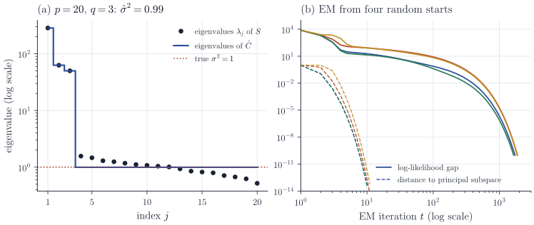
Panel (b) of Figure 1 separates two speeds. The column space of \(W_t\) converges in about ten iterations: the update multiplies \(W\) by \(S\) and then by a \(q \times q\) matrix, which is one step of subspace iteration, and the eigengap \(\lambda_3/\lambda_4\) is large here. The likelihood needs about two thousand iterations, because the lengths of the columns, which carry the estimates of \(\lambda_j - \sigma^2\), are corrected only by a small fraction per step when \(\lambda_j \gg \sigma^2\). For a single column, with \(\sigma^2\) held fixed, linearizing the update at the maximum gives a contraction factor of about \(1 - 2\sigma^2/\lambda_j\), which is \(0.993\) for the leading eigenvalue here. This is the familiar slowness of EM when the fraction of missing information is large: if the latent scores were observed, the noise level \(\sigma^2\) would pin down the loadings far more precisely than the observed data pin down their lengths when \(\lambda_j \gg \sigma^2\). It is a reason to prefer the closed form whenever it is available.
Remarks
Replacing \(\sigma^2 I_p\) by a general diagonal matrix gives the factor analysis model, which has no closed-form maximum likelihood estimate and is invariant to rescaling individual variables, unlike probabilistic PCA. The choice of \(q\) can be made with the maximized likelihood, which depends on the data only through the eigenvalues of \(S\), by penalized criteria or Bayesian model comparison; Bishop’s automatic relevance determination prior on the columns of \(W\) is one Bayesian route. Mixtures of probabilistic principal component analysers, fitted by EM, are developed in Tipping and Bishop, “Mixtures of probabilistic principal component analyzers” (Neural Computation, 1999).