Likelihood from two moments: quasi-likelihood and the variance function

The maximum likelihood equations of a generalized linear model have a curious feature. For any exponential dispersion family with mean $\mu_i(\beta)$ and variance $\phi V(\mu_i)$, they read

\[\sum_{i=1}^n \frac{\partial \mu_i(\beta)}{\partial \beta} \, \frac{y_i - \mu_i(\beta)}{\phi\, V(\mu_i(\beta))} = 0 ,\]

so the distribution enters only through its first two moments. Wedderburn (1974) proposed to take this equation as the definition of the estimator whenever a mean model and a variance function can be specified, whether or not they belong to an actual distribution. Counts whose variance is a multiple of the mean, continuous responses with constant coefficient of variation, and proportions that are not binomial counts all fit this pattern. The resulting theory is called quasi-likelihood. It rests on two facts: the estimating equation is unbiased whenever the mean model is correct, and among estimating equations linear in the data it is the most efficient when the variance function is correct.

The quasi-score of one observation

Let $Y$ have mean $\mu$ and variance $\phi V(\mu)$, where $V$ is a known positive, differentiable function on the range of $\mu$ and $\phi > 0$ is a dispersion parameter. Define the quasi-score

\[U(\mu; y) = \frac{y - \mu}{\phi V(\mu)} .\]

Lemma 1. $\E\, U(\mu; Y) = 0$ and $\Var U(\mu; Y) = -\E\, \dfrac{\partial U(\mu; Y)}{\partial \mu} = \dfrac{1}{\phi V(\mu)}$.

Proof. The first two claims follow from $\E Y = \mu$ and $\Var Y = \phi V(\mu)$. For the third, $\partial U / \partial \mu = -1/(\phi V(\mu)) - (y - \mu) V'(\mu)/(\phi V(\mu)^2)$, and the second term has mean zero.

These are the two properties of a genuine score $\partial_\mu \log p_\mu(y)$ on which likelihood asymptotics rest: it has mean zero at the true parameter, and its variance equals its expected negative derivative (the information identity). Here they hold by construction, using nothing beyond the two moments. Integrating the quasi-score gives the quasi-likelihood

\[Q(\mu; y) = \int_y^\mu \frac{y - t}{\phi V(t)} \, \dd t ,\]

which is normalized so that $Q(y; y) = 0$ and $Q \le 0$. The quasi-deviance $-2\phi \sum_i Q(\hat\mu_i; y_i)$ plays the role of the deviance. Elementary integration gives, up to the factor $1/\phi$:

$V(\mu) = 1$: $\; Q = -\tfrac12 (y - \mu)^2$, the normal log-likelihood in $\mu$;
$V(\mu) = \mu$: $\; Q = y \log(\mu/y) - (\mu - y)$, the Poisson form;
$V(\mu) = \mu^2$: $\; Q = -y/\mu - \log(\mu/y) + 1$, the gamma form;
$V(\mu) = \mu^3$: $\; Q = -y/(2\mu^2) + 1/\mu - 1/(2y)$, the inverse Gaussian form;
$V(\mu) = \mu(1 - \mu)$: $\; Q = y \log(\mu/y) + (1 - y)\log\bigl((1 - \mu)/(1 - y)\bigr)$, the binomial form for a proportion.

(The terms involving only $y$ come from the lower limit of integration. For $y = 0$ in the Poisson and binomial forms, and $y = 1$ in the binomial form, they are interpreted by continuity, with $0 \log 0 = 0$; the gamma and inverse Gaussian forms require $y > 0$.) In each case $Q$ coincides, as a function of $\mu$, with the log-likelihood of a familiar family. The point of the construction is that the quasi-likelihood may be used when that family is not credible: $V(\mu) = \mu$ for overdispersed counts with $\phi > 1$, or for nonnegative continuous data; $V(\mu) = \mu(1 - \mu)$ for proportions measured on a continuous scale.

Regression

Now let $Y_1, \dots, Y_n$ be independent with

\[\E Y_i = \mu_i(\beta), \qquad \Var Y_i = \phi V(\mu_i(\beta)), \qquad \beta \in \R^p,\]

and write $D_i(\beta) = \nabla_\beta\, \mu_i(\beta) \in \R^p$ and $V_i(\beta) = V(\mu_i(\beta))$. In a generalized linear model $\mu_i(\beta) = h(x_i^\top \beta)$ for an inverse link $h$, and $D_i = h'(x_i^\top \beta)\, x_i$. The quasi-score for $\beta$ is the chain-rule image of the single-observation quasi-scores,

\[U_n(\beta) = \sum_{i=1}^n D_i(\beta) \, \frac{Y_i - \mu_i(\beta)}{\phi\, V_i(\beta)} ,\]

and the quasi-likelihood estimator $\hat\beta$ solves $U_n(\hat\beta) = 0$. The dispersion $\phi$ cancels from the equation, so $\hat\beta$ does not depend on it; it is usually estimated afterwards from Pearson residuals, $\hat\phi = (n - p)^{-1} \sum_i (Y_i - \hat\mu_i)^2 / V(\hat\mu_i)$. Computationally, the equation is solved by Fisher scoring (iteratively reweighted least squares) exactly as for a generalized linear model.

The first-order behaviour of $\hat\beta$ follows from a one-term expansion of $U_n$ around the true value $\beta_0$:

\[0 = U_n(\hat\beta) \approx U_n(\beta_0) - \Omega_n (\hat\beta - \beta_0), \qquad \Omega_n = \sum_{i=1}^n \frac{D_i D_i^\top}{\phi V_i},\]

where the derivatives are evaluated at $\beta_0$. The matrix $\Omega_n$ is the expectation of $-\nabla_\beta U_n(\beta_0)$; the term of the derivative that involves $Y_i - \mu_i$ has mean zero and is negligible after scaling by $\Omega_n^{-1}$. Two consequences can be read off.

Only the mean has to be right for consistency. The expansion is centred because $\E\, U_n(\beta_0) = 0$, and this uses only $\E Y_i = \mu_i(\beta_0)$. A wrong variance function changes the weights in $U_n$, but the equation remains unbiased.
The variance has to be right for the usual standard errors. In general $\Cov U_n(\beta_0) = \sum_i D_i D_i^\top \Var(Y_i) / (\phi V_i)^2$, and

\[\Cov(\hat\beta) \approx \Omega_n^{-1} \Bigl( \sum_{i=1}^n \frac{D_i D_i^\top \Var(Y_i)}{\phi^2 V_i^2} \Bigr) \Omega_n^{-1} ,\]

which reduces to $\Omega_n^{-1} = \phi \bigl(\sum_i D_i D_i^\top / V_i\bigr)^{-1}$ if $\Var Y_i = \phi V_i$, by the information identity of Lemma 1 summed over observations.

Making the approximations rigorous requires regularity conditions on the sequence of designs: identifiability, eigenvalues of $\Omega_n / n$ bounded away from zero and infinity, smoothness of $\mu_i$ and $V$ in a neighbourhood of $\beta_0$ uniformly in $i$, and a Lindeberg condition for $U_n(\beta_0)$, for instance uniformly bounded moments of order $2 + \delta$. Under such conditions $\hat\beta$ is consistent and asymptotically normal with the covariance above; McCullagh (1983) gives a careful treatment. The sandwich form is estimated by replacing $\Var(Y_i)$ with $(Y_i - \hat\mu_i)^2$, as in the generalized estimating equations of Liang and Zeger.

Optimality

Why use the weights $D_i / V_i$ rather than some other choice? Consider any estimating function that is linear in the data,

\[g_n(\beta) = \sum_{i=1}^n a_i(\beta) \bigl(Y_i - \mu_i(\beta)\bigr), \qquad a_i(\beta) \in \R^p \text{ nonrandom}.\]

It is unbiased whenever the mean model is correct, and the same expansion shows that its root has approximate covariance

\[\Lambda(a) = (A^\top D)^{-1} A^\top \Sigma A (D^\top A)^{-1},\]

where $A$ and $D$ are the $n \times p$ matrices with rows $a_i^\top$ and $D_i^\top$ at $\beta_0$, $\Sigma = \diag(\Var Y_1, \dots, \Var Y_n)$, and $A^\top D$ is assumed nonsingular.

Theorem 2. Assume $\Sigma$ is positive definite and $D$ has full column rank. For every admissible $A$,

\[\Lambda(a) \succeq (D^\top \Sigma^{-1} D)^{-1}\]

in the positive semidefinite order, with equality if and only if $A = \Sigma^{-1} D C$ for some nonsingular $p \times p$ matrix $C$. In particular, if $\Var Y_i = \phi V(\mu_i)$, the quasi-score has the smallest asymptotic covariance among all linear unbiased estimating functions.

Proof. Put $B_0 = (D^\top \Sigma^{-1} D)^{-1} D^\top \Sigma^{-1}$ and $B = (A^\top D)^{-1} A^\top$, both $p \times n$. Then $B D = B_0 D = I_p$, so $M = B - B_0$ satisfies $M D = 0$. Since $\Lambda(a) = B \Sigma B^\top$,

\[\Lambda(a) = B_0 \Sigma B_0^\top + M \Sigma M^\top + B_0 \Sigma M^\top + M \Sigma B_0^\top .\]

The cross terms vanish: $B_0 \Sigma M^\top = (D^\top \Sigma^{-1} D)^{-1} (M D)^\top = 0$. Also $B_0 \Sigma B_0^\top = (D^\top \Sigma^{-1} D)^{-1}$. Hence $\Lambda(a) - (D^\top \Sigma^{-1} D)^{-1} = M \Sigma M^\top \succeq 0$, with equality if and only if $M = 0$, because $\Sigma$ is positive definite. Finally, $M = 0$ means $A^\top = (A^\top D)(D^\top \Sigma^{-1} D)^{-1} D^\top \Sigma^{-1}$, that is, $A = \Sigma^{-1} D C$ with $C = (D^\top \Sigma^{-1} D)^{-1} (D^\top A)$, which is nonsingular; the converse is immediate.

The argument is the Gauss–Markov theorem in the language of estimating equations. Optimality results of this kind go back to Godambe (1960) and are developed systematically in Heyde’s book cited below. Quasi-likelihood thus solves an optimization problem posed entirely in terms of first and second moments. If the variance function is wrong, the estimator remains consistent but loses efficiency, and its model-based standard errors are wrong.

A misspecified variance function

To see the size of these effects, take $n = 200$ observations with $x_i$ equally spaced on $[0, 3]$, log link $\mu_i = \exp(\beta_0 + \beta_1 x_i)$ with $(\beta_0, \beta_1) = (0.5, 1)$, and gamma responses with $\Var Y_i = 0.5\, \mu_i^2$, a constant coefficient of variation. Fit the slope by quasi-likelihood with working variance $V(\mu) = \mu^q$ for several powers $q$. For the log link, $D_i = \mu_i z_i$ with $z_i = (1, x_i)^\top$, and $\Lambda(a)$ can be evaluated exactly with $a_i = \mu_i^{1-q} z_i$.

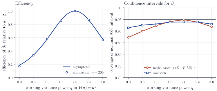
Left: efficiency of the slope estimator as a function of the working variance power. Right: coverage of model-based and sandwich intervals as a function of the working variance power. — Figure 1. Gamma responses with $\mathrm{Var}\,Y = 0.5\,\mu^2$ and log link, fitted with working variance $V(\mu) = \mu^q$. Left: asymptotic efficiency $\Lambda_{22}(q = 2)/\Lambda_{22}(q)$ of $\hat\beta_1$ (curve) and the ratio of Monte Carlo variances over $2000$ replications (circles). Right: coverage of nominal $95\%$ Wald intervals using the model-based covariance with Pearson $\hat\phi$, and the sandwich covariance.

The left panel confirms Theorem 2: efficiency is maximal at the true power $q = 2$ and decays on both sides. Using Poisson-type weights ($q = 1$) costs about $40\%$ of the efficiency, and unweighted nonlinear least squares ($q = 0$) more than $80\%$, because it gives the largest weight to the observations with the largest variance. The right panel shows the second consequence. Rescaling by $\hat\phi$ corrects the overall level of the variance but not its shape, so model-based intervals undercover when $q$ is far from $2$. The sandwich intervals are much less sensitive to $q$, with coverage between $0.91$ and $0.94$; the remaining shortfall reflects the downward bias of the sandwich variance estimator in moderate samples, and it is largest for small $q$, where a few high-variance observations carry most of the weight.

Remarks

The most common application is to overdispersed counts with $V(\mu) = \mu$ and $\phi > 1$, often called quasi-Poisson regression. The estimates coincide with the Poisson maximum likelihood estimates; only the standard errors are multiplied by $\hat\phi^{1/2}$. Overdispersion of the negative binomial type, $\Var Y = \mu + \mu^2/k$, has a different variance function, and Figure 1 suggests that the choice matters more for efficiency than for validity.

Choosing $V$ is a modelling decision. Plots of squared Pearson residuals against fitted values are informative, and the extended quasi-likelihood of Nelder and Pregibon (1987) adds a term that allows variance functions to be compared by a likelihood-like criterion. For correlated responses, the quasi-score $D^\top V^{-1} (y - \mu)$ with a nondiagonal working covariance $V$ is in general not the gradient of any function, so a quasi-likelihood need not exist; the estimating equation, which is all the theory above uses, still does.

References: V. P. Godambe, “An optimum property of regular maximum likelihood estimation”, Annals of Mathematical Statistics (1960); R. W. M. Wedderburn, “Quasi-likelihood functions, generalized linear models, and the Gauss–Newton method”, Biometrika (1974); P. McCullagh, “Quasi-likelihood functions”, Annals of Statistics (1983); K.-Y. Liang and S. L. Zeger, “Longitudinal data analysis using generalized linear models”, Biometrika (1986); McCullagh and Nelder, Generalized Linear Models, 2nd edition (1989); C. C. Heyde, Quasi-Likelihood and Its Application (1997).