Random Fourier features: approximating a kernel by sampling its spectral measure

Kernel methods need the $n \times n$ Gram matrix, and the costs of forming, storing and factorizing it grow like $n^2$ and $n^3$. Rahimi and Recht (Random features for large-scale kernel machines, NIPS 2007) proposed replacing a shift-invariant kernel by the inner product of an explicit random feature map $z : \R^d \to \R^D$, chosen so that $\E\, z(x)^\top z(x') = k(x, x')$. Linear methods applied to $z(x)$ then approximate the kernel method at a cost linear in $n$. The construction rests on Bochner’s theorem, which identifies such kernels with probability measures; the error of the approximation is then a Monte Carlo error, and its size depends on the number of features and on the tails of that measure.

Bochner’s theorem

A kernel on $\R^d$ is shift-invariant if $k(x, x') = \kappa(x - x')$ for a function $\kappa : \R^d \to \R$. Symmetry of the kernel means $\kappa(-\delta) = \kappa(\delta)$. It is positive definite (in the sense of producing positive semidefinite Gram matrices) when $\sum_{j,l} c_j c_l\, \kappa(x_j - x_l) \ge 0$ for all finite collections of points and real coefficients. Since a real symmetric matrix is positive semidefinite over $\mathbb C$ as soon as it is over $\R$, the same inequality then holds with $c_j\bar c_l$ for complex coefficients.

Theorem 1 (Bochner). A continuous function $\kappa : \R^d \to \mathbb C$ is positive definite if and only if there is a finite non-negative Borel measure $\mu$ on $\R^d$ with

\[\kappa(\delta) = \int_{\R^d} e^{i\omega^\top\delta}\, \mu(\dd\omega), \qquad \delta \in \R^d .\]

The measure is unique, and $\mu(\R^d) = \kappa(0)$.

The “if” direction is a one-line computation: for complex $c_1, \dots, c_n$ and points $x_1, \dots, x_n$,

\[\sum_{j,l} c_j \bar c_l\, \kappa(x_j - x_l) = \int \sum_{j,l} c_j e^{i\omega^\top x_j}\, \overline{c_l e^{i\omega^\top x_l}}\, \mu(\dd\omega) = \int \Bigl\lvert \sum_j c_j e^{i\omega^\top x_j}\Bigr\rvert^2 \mu(\dd\omega) \ge 0 .\]

The converse is the substance of the theorem; proofs can be found in Rudin, Fourier Analysis on Groups (1962), and in Wendland, Scattered Data Approximation (2005). Normalizing $\kappa(0) = 1$ makes $\mu$ a probability measure, the spectral measure of the kernel, and $\kappa$ is its characteristic function. When $\kappa$ is real, uniqueness of $\mu$ and $\kappa(-\delta) = \overline{\kappa(\delta)} = \kappa(\delta)$ force $\mu$ to be symmetric, and then

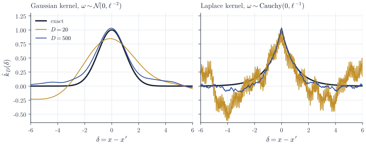
\[\kappa(\delta) = \E\cos(\omega^\top\delta), \qquad \omega \sim \mu .\]

Two examples in one dimension: the Gaussian kernel $\kappa(\delta) = e^{-\delta^2/(2\ell^2)}$ is the characteristic function of $\mathcal N(0, \ell^{-2})$, and the Laplace kernel $\kappa(\delta) = e^{-\abs{\delta}/\ell}$ is that of the Cauchy distribution with scale $\ell^{-1}$. Smoothness of the kernel at the origin corresponds to tails of the spectral measure: the Gaussian kernel is analytic and its spectral measure has all moments, while the Laplace kernel has a corner at $0$ and its spectral measure has no mean.

Random features

Draw $\omega_1, \dots, \omega_D$ independently from $\mu$ and $b_1, \dots, b_D$ independently from the uniform distribution on $[0, 2\pi)$, and set

\[z(x) = \sqrt{\tfrac{2}{D}}\,\bigl(\cos(\omega_1^\top x + b_1), \dots, \cos(\omega_D^\top x + b_D)\bigr), \qquad \hat k_D(x, x') = z(x)^\top z(x').\]

A variant without phases uses $D/2$ frequencies and the pairs $(\cos\omega_j^\top x, \sin\omega_j^\top x)$, scaled by $\sqrt{2/D}$, so that $\hat k_D(x,x') = \frac2D \sum_{j=1}^{D/2}\cos\bigl(\omega_j^\top(x - x')\bigr)$ by the subtraction formula for the cosine. Both are averages of independent bounded terms.

Proposition 2. Let $\delta = x - x'$. Both estimators are unbiased, $\E\hat k_D(x, x') = \kappa(\delta)$, with variances

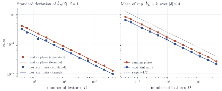
\[\Var \hat k_D^{\,\mathrm{phase}} = \frac{1}{D}\Bigl(1 + \tfrac12\kappa(2\delta) - \kappa(\delta)^2\Bigr), \qquad \Var \hat k_D^{\,\mathrm{pair}} = \frac{1}{D}\Bigl(1 + \kappa(2\delta) - 2\kappa(\delta)^2\Bigr).\]

Moreover, for every $\varepsilon > 0$, $\P\bigl(\abs{\hat k_D^{\,\mathrm{phase}} - \kappa(\delta)} \ge \varepsilon\bigr) \le 2e^{-D\varepsilon^2/8}$ and $\P\bigl(\abs{\hat k_D^{\,\mathrm{pair}} - \kappa(\delta)} \ge \varepsilon\bigr) \le 2e^{-D\varepsilon^2/4}$.

Proof. For one random-phase term, the product formula gives

\[Y = 2\cos(\omega^\top x + b)\cos(\omega^\top x' + b) = \cos(\omega^\top\delta) + \cos\bigl(\omega^\top(x + x') + 2b\bigr).\]

Given $\omega$, the angle $\omega^\top(x+x') + 2b$ is uniform modulo $2\pi$, so the second cosine has conditional mean $0$ and conditional second moment $\tfrac12$. Hence $\E[Y\mid\omega] = \cos(\omega^\top\delta)$, $\Var(Y\mid\omega) = \tfrac12$, and $\E Y = \kappa(\delta)$. By the law of total variance and $\cos^2 u = \tfrac12(1 + \cos 2u)$,

\[\Var Y = \tfrac12 + \Var\cos(\omega^\top\delta) = \tfrac12 + \tfrac12\bigl(1 + \kappa(2\delta)\bigr) - \kappa(\delta)^2 ,\]

and $\hat k_D^{\,\mathrm{phase}}$ is the average of $D$ independent copies of $Y$. For the paired features each of the $D/2$ terms is $\cos(\omega_j^\top\delta)$, with mean $\kappa(\delta)$ and variance $\tfrac12(1 + \kappa(2\delta)) - \kappa(\delta)^2$. The tail bounds are Hoeffding’s inequality for averages of $D$ independent terms in $[-2, 2]$ and of $D/2$ independent terms in $[-1, 1]$, respectively.

The difference of the two variances is $D^{-1}\bigl(\kappa(\delta)^2 - \tfrac12\kappa(2\delta)\bigr)$. For the Gaussian kernel $\kappa(2\delta) = \kappa(\delta)^4 \le \kappa(\delta)^2$, so the paired features are uniformly better at the same feature budget; the random phase adds the noise of the term $\cos(\omega^\top(x + x') + 2b)$, which carries no information about the kernel. Sutherland and Schneider (On the error of random Fourier features, UAI 2015) compare the two constructions in detail.

Random Fourier feature approximations of the Gaussian and Laplace kernels with twenty and five hundred features — Figure 1. Exact kernels (length-scale $\ell = 1$) and single random-phase approximations $\hat k_D(\delta, 0)$ with $D = 20$ and $D = 500$. The Gaussian approximations are smooth because the sampled frequencies are moderate; the Laplace approximations oscillate because Cauchy frequencies are occasionally very large.

How many features

Proposition 2 gives the pointwise rate $D^{-1/2}$ for every kernel, with a constant that does not depend on the dimension $d$. Figure 2 confirms the variance formulas for the Gaussian kernel and shows that the error of the whole function $\delta \mapsto \hat k_D(\delta)$ over a bounded interval decreases at the same rate. Uniform control over a compact set $M \subset \R^d$ requires more than the pointwise bound, since the estimator must be accurate at infinitely many pairs simultaneously. Rahimi and Recht prove such a bound with a covering argument and Lipschitz control of $\hat k_D - \kappa$; the Lipschitz constant involves $\sigma_\mu^2 = \E\norm{\omega}^2$, and the resulting requirement is a number of features of order $d\,\varepsilon^{-2}\log(\sigma_\mu \operatorname{diam} M/\varepsilon)$ for uniform error $\varepsilon$ with high probability. The bound needs $\sigma_\mu < \infty$, which fails for the Laplace kernel; the rough approximations on the right of Figure 1 are the visible symptom.

Standard deviation of the kernel estimate at one point and mean supremum error against the number of features, on log-log axes — Figure 2. Gaussian kernel with $\ell = 1$, 400 replications for each $D$. Left: standard deviation of $\hat k_D(\delta)$ at $\delta = 1$ for random-phase features and for $(\cos,\sin)$ pairs with the same total number of features, simulated (markers) and from Proposition 2 (lines). Right: average over replications of the maximum error on $\lvert\delta\rvert \le 4$, with a reference line of slope $-1/2$.

Using the features

With the $n \times D$ feature matrix $Z$ whose rows are $z(x_i)^\top$, the Gram matrix is approximated by $ZZ^\top$, a matrix of rank at most $D$. Kernel ridge regression with the approximate kernel becomes ridge regression on the features,

\[\hat\beta = (Z^\top Z + n\lambda I_D)^{-1}Z^\top y, \qquad \hat f(x) = z(x)^\top\hat\beta,\]

at a cost of $O(nD^2 + D^3)$ time and $O(nD)$ memory instead of $O(n^3)$ and $O(n^2)$. The approximation error of the Gram matrix is not the right measure of success for this use: what matters is the excess risk of $\hat f$. Rudi and Rosasco (Generalization properties of learning with random features, NeurIPS 2017) show that for kernel ridge regression, under standard regularity conditions, a number of features of order $\sqrt n \log n$ already preserves the learning rate of the exact estimator.

Remarks

The construction is Monte Carlo integration of $\kappa(\delta) = \E\cos(\omega^\top\delta)$, and the usual variance-reduction ideas apply: replacing independent frequencies by orthogonal or quasi-Monte Carlo ones reduces the error for the Gaussian kernel. The same idea extends to kernels that are not shift-invariant whenever the kernel has an integral representation $k(x, x') = \E[\phi(x, \omega)\phi(x', \omega)]$, for example dot-product kernels and the arc-cosine kernels associated with infinitely wide neural networks. For non-shift-invariant kernels Bochner’s theorem no longer applies, and the representation must be found case by case.