Is the random seed a tuning parameter? Seed variability and the optimism of the best seed
Setting a random seed makes a computation reproducible: run it twice and the output is identical. This is valuable, and it is easy to forget that the output is still random. A different seed would have produced a different initialization, a different order of stochastic gradient steps, a different train–test split, or a different Markov chain, and therefore, in general, a different answer. The question in the title has a precise answer once the computation is written as a randomized procedure, and the answer separates legitimate uses of several seeds from illegitimate ones.
A computation as a randomized procedure
Write the output of an analysis as
\[T = t(D, U),\]where \(D\) is the data, \(U\) is the auxiliary randomness consumed by the algorithm, and \(t\) is a fixed measurable function. A pseudo-random generator maps a seed \(s\) to a stream \(U_s\). We adopt the standard idealization that streams from different seeds behave like independent draws from a fixed distribution, independent of \(D\). A seed is then a label for one realization of \(U\), and fixing it is conditioning on that realization.
If \(\E T^2 < \infty\), the law of total variance splits the variability of the output into two parts,
\[\Var T = \underbrace{\E\bigl[\Var(T \mid D)\bigr]}_{\text{seed}} + \underbrace{\Var\bigl(\E[T \mid D]\bigr)}_{\text{data}} .\]The first term is internal to the algorithm: it would remain if the data were held fixed. Reproducing a computation with the same seed hides it completely, while reproducing the study with new data would expose both terms. Reporting results from a single seed treats the first term as if it were zero.
The size of the seed term varies enormously between procedures. It is exactly zero for least squares solved by a direct method and negligible for a well-mixed long MCMC run, but it can dominate for nonconvex optimization and for evaluations based on a single small test set. Two simulated examples show the last two cases.
Two examples
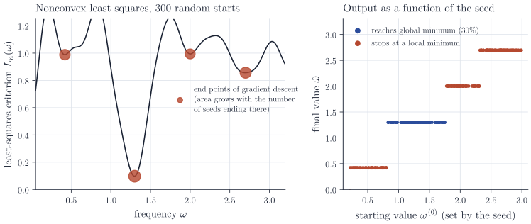
Random starting values. Let \(y_i = \sin(1.3\, x_i) + \varepsilon_i\), \(i = 1, \dots, 100\), with \(x_i\) uniform on \((0, 10)\) and \(\varepsilon_i \sim N(0, 0.3^2)\), and estimate the frequency by minimizing \(L_n(\omega) = n^{-1}\sum_i \{y_i - \sin(\omega x_i)\}^2\) with gradient descent from a starting value drawn uniformly on \((0.2, 3)\). The criterion has many local minima, because \(\sin(\omega x_i)\) is periodic in \(\omega\) for each \(x_i\), and gradient descent converges to the one whose basin contains the starting value. In Figure 1, only \(30\%\) of the seeds lead to the global minimum near \(\omega = 1.3\); the rest return one of several poor local fits. The output is a step function of the starting value, and the seed decides which step.
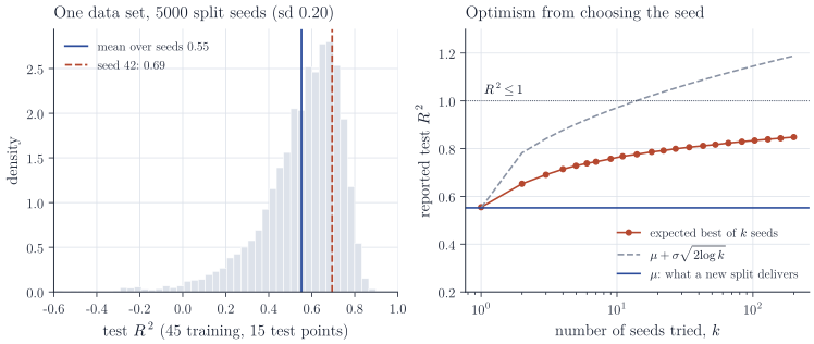
Random train–test splits. Take \(n = 60\) observations from a linear model with eight predictors, fit least squares on \(45\) of them and compute \(R^2\) on the remaining \(15\). The data set is fixed, and the only randomness is which \(15\) points form the test set. Over \(5000\) split seeds, the test \(R^2\) has mean \(0.55\) and standard deviation \(0.20\); its \(5\%\) and \(95\%\) quantiles are \(0.19\) and \(0.78\) (Figure 2, left). With the conventional seed \(42\) the reported value would have been \(0.69\). None of this spread reflects a difference between models. It is entirely the conditional variance \(\Var(T \mid D)\) of the evaluation.
Averaging over seeds
If \(T_1, \dots, T_m\) are computed from the same data with independent streams \(U_1, \dots, U_m\), they are conditionally independent and identically distributed given \(D\), so
\[\Var\Bigl(\frac1m \sum_{j=1}^m T_j\Bigr) = \frac{\E\bigl[\Var(T \mid D)\bigr]}{m} + \Var\bigl(\E[T \mid D]\bigr).\]Averaging removes the seed term at rate \(1/m\) and leaves the data term untouched. Repeated random splitting and repeated cross-validation are instances of this formula, as are ensembles over random initializations. The spread of the \(T_j\) estimates the seed term, \(\E[\Var(T \mid D)]\) for the data at hand, and should be reported with the average.
The same reasoning applies to comparisons. To compare procedures \(A\) and \(B\), run both with the same seeds, so that they see the same splits or the same streams. Then
\[\Var(T_A - T_B \mid D) = \Var(T_A \mid D) + \Var(T_B \mid D) - 2\Cov(T_A, T_B \mid D),\]and the covariance induced by the shared randomness is typically large and positive: a split with hard test points is hard for both methods. This is the method of common random numbers from simulation.
Choosing the seed
Suppose \(k\) seeds are tried and the best result is reported. Whether this is legitimate depends on where the seed enters and what data the choice uses.
If the seed enters only the evaluation, as with the split above, choosing it does not change the fitted model at all. It selects a favourable test set, and the selected value is biased upward. The size of the bias does not require independence between seeds.
Proposition 1. Let \(S_1, \dots, S_k\) have common mean \(\mu\) and satisfy \(\E e^{\lambda(S_j - \mu)} \le e^{\lambda^2\sigma^2/2}\) for all \(\lambda > 0\) and all \(j\). Then
\[\E \max_{j \le k} S_j \le \mu + \sigma\sqrt{2\log k}.\]Proof. For \(\lambda > 0\), Jensen’s inequality, the bound of a maximum of nonnegative terms by their sum, and the assumption give
\[\exp\Bigl(\lambda\, \E \max_j (S_j - \mu)\Bigr) \le \E \exp\Bigl(\lambda \max_j (S_j - \mu)\Bigr) \le \sum_{j=1}^k \E e^{\lambda(S_j - \mu)} \le k\, e^{\lambda^2 \sigma^2/2}.\]Taking logarithms, \(\E\max_j(S_j - \mu) \le (\log k)/\lambda + \lambda\sigma^2/2\), and the choice \(\lambda = \sqrt{2\log k}/\sigma\) gives the bound.
The bound has the right order: for independent normal \(S_j\) with variance \(\sigma^2\), \(\E\max_j S_j - \mu\) is asymptotic to \(\sigma\sqrt{2\log k}\) as \(k \to \infty\). For the split example, the best of \(10\) seeds has expected test \(R^2\) of about \(0.76\) and the best of \(100\) about \(0.83\), against the honest value \(0.55\) (Figure 2, right). The dashed curve in Figure 2 is \(\mu + \sigma\sqrt{2\log k}\) with \(\sigma\) the observed standard deviation; it would be a valid bound if the split distribution were sub-Gaussian with variance proxy equal to its variance, as for a normal distribution. The actual values lie well below it, because \(R^2\) is at most one and its distribution over splits is skewed to the left with a short upper tail. The optimism is nevertheless larger than any plausible difference between competing methods on data of this size. On new data, the model fitted on the chosen split has no systematic advantage over one fitted on a random split: the advantage belonged to the test set, not to the model.
If the seed enters the fitting, as with the starting value in Figure 1, the situation is different. Running gradient descent from \(k\) starting values and keeping the solution with the smallest training criterion is a well-defined algorithm, the familiar multi-start strategy, and in the example it finds the global minimum with probability \(1 - 0.7^k\) under the idealization of independent starts. Selecting among the \(k\) fits by a validation criterion is also legitimate model selection. What is not legitimate is to select the seed by the same data used to report performance: then Proposition 1 applies to the reported number.
The formal answer to the title is therefore negative. A tuning parameter \(\lambda\) indexes a family of procedures \(t_\lambda\) whose distributions differ, and choosing \(\lambda\) well changes what can be expected on new data. Under the idealization above, all seeds give the same distribution of \(T\); there is nothing to tune, only a draw to condition on. A deterministic rule that uses several seeds, such as multi-start optimization or averaging, defines a new procedure, and that procedure can be better than a single run. It should be described and evaluated as such.
Remarks
The idealization that different seeds give independent streams is a property of good generators and should not be taken for granted for related seeds such as \(1, 2, 3, \dots\) in older generators; modern libraries provide explicit mechanisms for spawning independent streams. The optimism in Proposition 1 is the same phenomenon as the winner’s curse in multiple testing and the selection bias in reporting the best of many tuned models; the remedy in all cases is to keep the data used for selection separate from the data used for reporting.