Conditioning out the noise: Rao–Blackwellization of Monte Carlo estimators
The Rao–Blackwell theorem is usually met in estimation theory: conditioning an unbiased estimator on a sufficient statistic gives an unbiased estimator that is at least as good. The same operation is useful whenever an estimator is built from simulated random variables, some of whose randomness can be integrated out analytically. If a simulation produces pairs \((X, Y)\) and the target is \(\E h(X)\), then averaging \(m(Y) = \E[h(X) \mid Y]\) instead of \(h(X)\) removes the noise that \(X\) adds on top of \(Y\). For independent draws this never increases the variance. For Markov chain output the guarantee can fail, but in a two-block Gibbs sampler the gain can be computed exactly.
Conditioning reduces variance
Theorem 1. Let \(\delta\) be a random variable with \(\E \delta^2 < \infty\), let \(\mathcal G\) be a sub-\(\sigma\)-field, and put \(\delta^* = \E[\delta \mid \mathcal G]\). Then \(\E \delta^* = \E \delta\) and
\[\Var \delta = \Var \delta^* + \E\bigl[\Var(\delta \mid \mathcal G)\bigr] ,\]so \(\Var \delta^* \le \Var \delta\), with equality if and only if \(\delta\) is almost surely equal to a \(\mathcal G\)-measurable random variable.
Proof. The first claim is the tower property. Write \(\delta - \E\delta = (\delta - \delta^*) + (\delta^* - \E\delta)\). The cross term vanishes, since \(\delta^* - \E\delta\) is \(\mathcal G\)-measurable and square integrable (conditional expectation is a contraction in \(L^2\)), so
\[\E\bigl[(\delta - \delta^*)(\delta^* - \E\delta)\bigr] = \E\bigl[(\delta^* - \E\delta)\, \E[\delta - \delta^* \mid \mathcal G]\bigr] = 0 .\]Hence \(\Var\delta = \E(\delta - \delta^*)^2 + \Var\delta^*\), and \(\E(\delta - \delta^*)^2 = \E[\Var(\delta \mid \mathcal G)]\). Equality holds exactly when \(\delta = \delta^*\) almost surely.
In estimation theory \(\mathcal G\) is generated by a sufficient statistic \(T\), which guarantees that \(\E_\theta[\delta \mid T]\) does not depend on \(\theta\) and is therefore again an estimator; by the conditional Jensen inequality the conclusion extends from squared error to any loss convex in the estimate. In simulation there is no parameter to worry about. The only requirement is that the conditional expectation can be computed.
Independent draws
Let \((X_1, Y_1), \dots, (X_N, Y_N)\) be i.i.d. copies of \((X, Y)\), let \(h(X)\) be square integrable, and set \(m(y) = \E[h(X) \mid Y = y]\). Both
\[\hat\mu_N = \frac1N \sum_{i=1}^N h(X_i) \qquad \text{and} \qquad \tilde\mu_N = \frac1N \sum_{i=1}^N m(Y_i)\]are unbiased for \(\mu = \E h(X)\), and by Theorem 1 applied to one pair,
\[N \Var \hat\mu_N - N \Var \tilde\mu_N = \E\bigl[\Var(h(X) \mid Y)\bigr] \ge 0 .\]A small example shows the size of the effect. Let \(\Lambda \sim \mathrm{Gamma}(\alpha, \beta)\) (shape \(\alpha\), rate \(\beta\)) and \(X \mid \Lambda \sim \mathrm{Poisson}(\Lambda)\), and estimate \(p = \P(X = 0)\). The crude estimator averages the indicators \(\mathbf 1\{X_i = 0\}\), each with variance \(p(1 - p)\). Conditioning on \(\Lambda\) replaces each indicator by \(e^{-\Lambda_i}\). Using \(\E e^{-s\Lambda} = (\beta/(\beta + s))^\alpha\), we get \(p = (\beta/(\beta + 1))^\alpha\) and
\[\Var e^{-\Lambda} = \Bigl(\frac{\beta}{\beta + 2}\Bigr)^\alpha - \Bigl(\frac{\beta}{\beta + 1}\Bigr)^{2\alpha} .\]For \(\alpha = 2\), \(\beta = 1\) this is \(1/9 - 1/16 \approx 0.049\), against \(p(1 - p) = 3/16 \approx 0.188\) for the indicator: the conditioned estimator needs about one quarter of the simulation effort for the same precision. When computing \(m\) is expensive the comparison should be made per unit of computing time, but in conjugate models such as this one the conditional expectation costs almost nothing.
Dependent draws
Markov chain Monte Carlo produces dependent draws, and the relevant quantity becomes the asymptotic variance. For a stationary sequence \(f(Z_1), f(Z_2), \dots\) with autocovariances \(\gamma_f(k) = \Cov(f(Z_1), f(Z_{1+k}))\) satisfying \(\sum_k \abs{\gamma_f(k)} < \infty\),
\[N \Var\Bigl(\frac1N \sum_{t=1}^N f(Z_t)\Bigr) = \gamma_f(0) + 2\sum_{k=1}^{N-1}\Bigl(1 - \frac kN\Bigr)\gamma_f(k) \;\longrightarrow\; \sigma^2(f) = \gamma_f(0) + 2\sum_{k=1}^\infty \gamma_f(k),\]by dominated convergence for series. Conditioning reduces the lag-zero term \(\gamma(0)\), as in Theorem 1, but it changes the autocovariances as well, and nothing in Theorem 1 controls them. For general samplers the Rao–Blackwellized average can indeed have the larger asymptotic variance (Geyer, 1995, gives examples). There is one important case in which the comparison goes the right way, with an explicit margin.
Consider a two-block Gibbs sampler for a joint law \(\pi\) of \((X, Y)\). Starting from \(X_0\), it alternates
\[Y_t \sim \pi(y \mid X_{t-1}), \qquad X_t \sim \pi(x \mid Y_t), \qquad t = 1, 2, \dots\]Data augmentation algorithms, in which \(Y\) is a latent variable introduced to make both conditionals tractable, have this form.
Theorem 2. Suppose \(X_0 \sim \pi_X\), so that the chain is stationary, let \(h \in L^2(\pi_X)\) and \(m(y) = \E_\pi[h(X) \mid Y = y]\), and assume the autocovariances of \(m(Y_1), m(Y_2), \dots\) are absolutely summable. Then both \(\sigma^2_{\mathrm{crude}} = \sigma^2(h \circ X)\) and \(\sigma^2_{\mathrm{RB}} = \sigma^2(m \circ Y)\) exist, and
\[\sigma^2_{\mathrm{crude}} = \sigma^2_{\mathrm{RB}} + \Var_\pi h(X) + \Var_\pi m(Y) .\]Proof. Write \(\gamma_X(k) = \Cov(h(X_0), h(X_k))\) and \(\gamma_Y(k) = \Cov(m(Y_1), m(Y_{1+k}))\); by stationarity these do not depend on the time origin. The interleaved sequence \(X_0, Y_1, X_1, Y_2, \dots\) is a Markov chain, and \((X_0, Y_1) \sim \pi\).
Fix \(k \ge 1\). Given \((X_0, Y_1, \dots, Y_k)\), the variable \(X_k\) has law \(\pi(\cdot \mid Y_k)\), so \(\E[h(X_k) \mid X_0, Y_1, \dots, Y_k] = m(Y_k)\) and
\[\gamma_X(k) = \Cov\bigl(h(X_0), m(Y_k)\bigr) .\]Next condition on \(Y_1\). By the Markov property, \(X_0\) and \((X_1, Y_2, X_2, \dots)\) are conditionally independent given \(Y_1\), and since \((X_0, Y_1) \sim \pi\), \(\E[h(X_0) \mid Y_1] = m(Y_1)\). Hence
\[\E\bigl[h(X_0)\, m(Y_k)\bigr] = \E\bigl[\E[h(X_0) \mid Y_1]\; \E[m(Y_k) \mid Y_1]\bigr] = \E\bigl[m(Y_1)\, m(Y_k)\bigr],\]where the last step is the tower property. Both sides have mean product \(\mu^2\), so \(\gamma_X(k) = \gamma_Y(k - 1)\) for every \(k \ge 1\). In particular the \(\gamma_X(k)\) are absolutely summable, and
\[\begin{aligned} \sigma^2_{\mathrm{crude}} &= \gamma_X(0) + 2\sum_{k=1}^\infty \gamma_Y(k - 1) = \Var h(X) + \gamma_Y(0) + \Bigl[\gamma_Y(0) + 2\sum_{j=1}^\infty \gamma_Y(j)\Bigr] \\ &= \Var h(X) + \Var m(Y) + \sigma^2_{\mathrm{RB}} , \end{aligned}\]since the bracket is \(\sigma^2_{\mathrm{RB}}\) by definition.
The gap is never smaller than \(\Var h(X)\), the variance of a single independent draw, so in absolute terms the Rao–Blackwellized average always gains at least one draw’s worth of variance per draw. The relative gain depends on mixing. For the bivariate normal with correlation \(\rho\) and \(h(x) = x\), the \(X\)-chain is an autoregression with coefficient \(\rho^2\), \(\sigma^2_{\mathrm{crude}} = (1 + \rho^2)/(1 - \rho^2)\), and \(\sigma^2_{\mathrm{RB}} = \rho^2 (1 + \rho^2)/(1 - \rho^2)\). The ratio \(\rho^2\) is close to one exactly when the chain mixes slowly, and then most of the variance comes from autocorrelation, which conditioning does not remove. Liu, Wong and Kong (1994) studied the covariance structure of such samplers in detail and proved that the Rao–Blackwellized estimator is better for two-block samplers.
Rao–Blackwellized densities
Conditioning also gives smooth estimates of marginal densities from sampler output. Under stationarity,
\[\hat\pi_X(x) = \frac1N \sum_{t=1}^N \pi(x \mid Y_t)\]is unbiased for \(\pi_X(x)\) at every \(x\), and integrating it over a set \(B\) gives the Rao–Blackwellized estimate of \(\pi_X(B)\), which by Theorem 2 with \(h = \mathbf 1_B\) has smaller asymptotic variance than the empirical frequency of \(\{X_t \in B\}\). This device was popularized by Gelfand and Smith (1990). Unlike a kernel estimate, it needs no bandwidth and it inherits the tail behaviour of the conditional densities.
The figure uses data augmentation for the Student \(t_3\) distribution. If \(Y \sim \mathrm{Gamma}(\nu/2, \text{rate } \nu/2)\) and \(X \mid Y \sim N(0, 1/Y)\), then \(X \sim t_\nu\), and \(Y \mid X \sim \mathrm{Gamma}\bigl((\nu + 1)/2, \text{rate } (\nu + X^2)/2\bigr)\). Both conditionals are standard, so the Gibbs sampler is the two-block scheme above. For \(h(x) = \mathbf 1\{x > 3\}\) the conditional expectation is \(m(y) = 1 - \Phi(3\sqrt y)\).
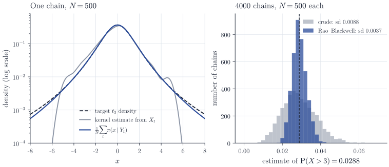
The numbers in the right panel check Theorem 2. The variance ratio is about \(5.6\). Theorem 2 predicts \(N(\Var\hat\mu_N - \Var\tilde\mu_N) \approx \Var h(X) + \Var m(Y)\), where \(\Var h(X) = p(1 - p) \approx 0.0280\) and a long simulation gives \(\Var m(Y) \approx 0.0032\), a total of \(0.0312\). The replicated chains give \(500 \times (0.00876^2 - 0.00371^2) \approx 0.0315\).
Remarks
The idea extends in several directions. In importance sampling and sequential Monte Carlo, integrating out a conditionally linear Gaussian part of the state analytically, with a Kalman filter, gives the Rao–Blackwellized particle filter. In Metropolis–Hastings algorithms, the rejected proposals carry information that can be recovered by conditioning; Casella and Robert (1996), “Rao–Blackwellisation of sampling schemes”, Biometrika, develop this. For samplers with more than two blocks, or with a random scan, the dependence structure no longer forces \(\gamma_X(k) = \gamma_Y(k - 1)\), and the comparison must be checked case by case.
The estimation-theory origins are C. R. Rao, “Information and the accuracy attainable in the estimation of statistical parameters”, Bulletin of the Calcutta Mathematical Society (1945), and D. Blackwell, “Conditional expectation and unbiased sequential estimation”, Annals of Mathematical Statistics (1947). For Markov chains: A. E. Gelfand and A. F. M. Smith, “Sampling-based approaches to calculating marginal densities”, Journal of the American Statistical Association (1990); J. S. Liu, W. H. Wong and A. Kong, “Covariance structure of the Gibbs sampler with applications to the comparisons of estimators and augmentation schemes”, Biometrika (1994); C. J. Geyer, “Conditioning in Markov chain Monte Carlo”, Journal of Computational and Graphical Statistics (1995).