Rare events that never stop: almost sure convergence versus convergence in probability

Two modes of convergence dominate asymptotic statistics. Consistency of an estimator is usually stated in probability, while laws of large numbers are often available in the stronger almost sure form. The two are easy to conflate because the standard examples converge in both senses. A single family of sequences separates them: independent indicators $X_n \sim \mathrm{Bernoulli}(p_n)$ with $p_n \to 0$ always converge to zero in probability, and converge almost surely exactly when $\sum_n p_n$ is finite.

Throughout, $X, X_1, X_2, \dots$ are real random variables on a probability space $(\Omega, \mathcal F, \P)$.

Definitions

The sequence $X_n$ converges to $X$ in probability, written $X_n \xrightarrow{p} X$, if for every $\varepsilon > 0$

\[\lim_{n\to\infty} \P\bigl(\abs{X_n - X} > \varepsilon\bigr) = 0 .\]

It converges almost surely, written $X_n \xrightarrow{\text{a.s.}} X$, if

\[\P\Bigl(\bigl\{\omega : \lim_{n\to\infty} X_n(\omega) = X(\omega)\bigr\}\Bigr) = 1 .\]

The first definition constrains each marginal law of $X_n - X$ separately; it says that at a large fixed time $n$ a deviation is unlikely. The second is a statement about entire sample paths $n \mapsto X_n(\omega)$: for almost every $\omega$, deviations eventually stop altogether. The set in the second definition is measurable, since

\[\bigl\{\lim_n X_n = X\bigr\} = \bigcap_{k \ge 1} \bigcup_{m \ge 1} \bigcap_{n \ge m} \bigl\{\abs{X_n - X} \le 1/k\bigr\},\]

a countable combination of events. The same identity gives a criterion that is easier to work with. Writing $A_n(\varepsilon) = \{\abs{X_n - X} > \varepsilon\}$ and

\[\limsup_{n} A_n(\varepsilon) = \bigcap_{m \ge 1} \bigcup_{n \ge m} A_n(\varepsilon) = \{\omega : \omega \in A_n(\varepsilon) \text{ for infinitely many } n\},\]

we have $X_n \xrightarrow{\text{a.s.}} X$ if and only if $\P(\limsup_n A_n(\varepsilon)) = 0$ for every $\varepsilon > 0$. (For the “if” direction it suffices to take $\varepsilon = 1/k$ and use countable subadditivity over $k$.)

Almost sure convergence implies convergence in probability

Proposition 1. If $X_n \xrightarrow{\text{a.s.}} X$, then $X_n \xrightarrow{p} X$.

Proof. Fix $\varepsilon > 0$ and let $B_m = \bigcup_{n \ge m} A_n(\varepsilon)$. The sets $B_m$ decrease to $\limsup_n A_n(\varepsilon)$, which has probability zero by the criterion above. Continuity of $\P$ from above gives $\P(B_m) \to 0$, and $\P(A_m(\varepsilon)) \le \P(B_m)$ because $A_m(\varepsilon) \subseteq B_m$.

The proof shows what is lost in passing from one mode to the other. Almost sure convergence controls the probability of a deviation at some time after $m$; convergence in probability controls only the probability of a deviation at time $m$.

Independent indicators

Let $X_1, X_2, \dots$ be independent with $X_n \sim \mathrm{Bernoulli}(p_n)$ and $p_n \to 0$. For $0 < \varepsilon < 1$ we have $A_n(\varepsilon) = \{X_n = 1\}$ with $X = 0$, so

\[\P(\abs{X_n} > \varepsilon) = p_n \to 0,\]

and $X_n \xrightarrow{p} 0$ whatever the rate at which $p_n$ vanishes. Almost sure convergence is a different matter: $X_n(\omega) \to 0$ exactly when only finitely many of the events $\{X_n = 1\}$ occur, because the sequence takes values in $\{0, 1\}$. Both directions are settled by the Borel–Cantelli lemmas.

Lemma 2 (Borel–Cantelli). Let $E_1, E_2, \dots$ be events.

If $\sum_n \P(E_n) < \infty$, then $\P(\limsup_n E_n) = 0$.
If the $E_n$ are independent and $\sum_n \P(E_n) = \infty$, then $\P(\limsup_n E_n) = 1$.

Proof. For part 1, $\P(\limsup_n E_n) \le \P\bigl(\bigcup_{n \ge m} E_n\bigr) \le \sum_{n \ge m} \P(E_n)$ for every $m$, and the right-hand side is the tail of a convergent series.

For part 2 it suffices to show $\P\bigl(\bigcap_{n \ge m} E_n^c\bigr) = 0$ for each $m$. By independence and the inequality $1 - x \le e^{-x}$, for every $M \ge m$,

\[\P\Bigl(\bigcap_{n=m}^{M} E_n^c\Bigr) = \prod_{n=m}^{M} \bigl(1 - \P(E_n)\bigr) \le \exp\Bigl(-\sum_{n=m}^{M} \P(E_n)\Bigr).\]

The exponent tends to $-\infty$ as $M \to \infty$, and continuity from above finishes the argument.

Applied to $E_n = \{X_n = 1\}$, the lemma gives a complete answer for independent indicators:

\[X_n \xrightarrow{\text{a.s.}} 0 \iff \sum_{n} p_n < \infty .\]

With $p_n = 1/n$ the harmonic series diverges, so with probability one the sequence equals $1$ infinitely often. Since $\sum_n (1 - p_n) = \infty$ as well, it also equals $0$ infinitely often, so it converges to zero in probability and almost surely does not converge to anything. With $p_n = 1/n^2$ the series converges, and almost every path is eventually identically zero.

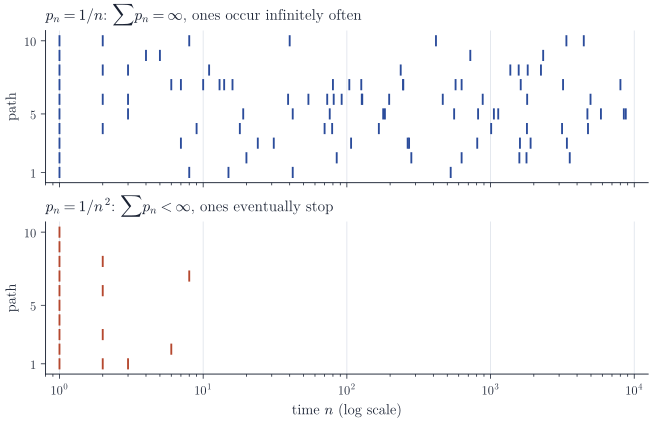
Sample paths of independent indicators with success probabilities one over n and one over n squared — Figure 1. Times $n \le 10^4$ at which $X_n = 1$, for ten independent paths of each sequence (horizontal axis on a log scale). With $p_n = 1/n$ (top) new ones keep appearing on every path, at a roughly constant rate per decade of $n$, since $\sum_{n=a}^{10a} 1/n \approx \log 10$. With $p_n = 1/n^2$ (bottom) each path has a last one, typically early.

The figure makes the mechanism visible. Under $p_n = 1/n$ the expected number of ones between $a$ and $10a$ is close to $\log 10 \approx 2.3$ for every $a$, so the ones thin out on the linear scale but never stop. Convergence in probability sees only the thinning.

Independence is essential in the second half of the equivalence. Let $U$ be uniform on $(0, 1)$ and $Y_n = \mathbf 1\{U \le 1/n\}$. Each $Y_n$ is again $\mathrm{Bernoulli}(1/n)$, so the marginal laws are exactly those of the first example, but now $Y_n(\omega) = 0$ for all $n > 1/U(\omega)$, and $Y_n \to 0$ almost surely. Convergence in probability depends only on the marginal laws of the $X_n - X$; almost sure convergence depends on their joint law, and part 2 of Lemma 2 is where the joint law enters. Summability of $\P(\abs{X_n - X} > \varepsilon)$ for every $\varepsilon > 0$ is therefore sufficient for almost sure convergence, by part 1, but not necessary.

What survives: subsequences

Convergence in probability does carry some pathwise information. The divergence in the example above is caused by summing $p_n$ over all $n$; along a sparse subsequence the sum can be made finite.

Proposition 3. If $X_n \xrightarrow{p} X$, there is a deterministic subsequence $n_1 < n_2 < \cdots$ with $X_{n_k} \xrightarrow{\text{a.s.}} X$.

Proof. Choose $n_k > n_{k-1}$ such that $\P(\abs{X_{n_k} - X} > 2^{-k}) \le 2^{-k}$, which is possible by convergence in probability. By part 1 of Lemma 2, almost surely $\abs{X_{n_k} - X} \le 2^{-k}$ for all but finitely many $k$, and on that event $X_{n_k} \to X$.

For the indicators with $p_n = 1/n$, the subsequence $n_k = k^2$ already works, since $\sum_k 1/k^2 < \infty$.

Proposition 3 also yields a useful characterization: $X_n \xrightarrow{p} X$ if and only if every subsequence has a further subsequence converging to $X$ almost surely. The “only if” part is Proposition 3 applied to the subsequence. For the converse, if $X_n$ did not converge in probability there would be $\varepsilon, \delta > 0$ and a subsequence along which $\P(\abs{X_n - X} > \varepsilon) \ge \delta$; no further subsequence could converge almost surely, by Proposition 1. It also shows that almost sure convergence is not induced by any topology on the space of random variables. In a topological space a sequence converges to $x$ whenever every subsequence has a further subsequence converging to $x$; a topology for almost sure convergence would therefore make it coincide with convergence in probability, which the indicators with $p_n = 1/n$ rule out. Convergence in probability, by contrast, is metrizable, for instance by $d(X, Y) = \E \min(\abs{X - Y}, 1)$.

Remarks

The example is not pathological from a statistical point of view. A sequential test that rejects at time $n$ with probability $\alpha_n \to 0$ under the null, using independent data at each time, has vanishing size at each fixed $n$; yet if $\sum_n \alpha_n = \infty$ it rejects infinitely often with probability one. This is the reason that guarantees for continuously monitored procedures must be stated uniformly over time, and why the distinction between the two modes of convergence matters in practice.

Two standard references for this material are Chapter 2 of Durrett, Probability: Theory and Examples, and Chapter 7 of Grimmett and Stirzaker, Probability and Random Processes.