The representer theorem: why kernel ridge regression lives in the span of the data
Fitting a function by penalized least squares over a rich function space looks like an infinite-dimensional optimization problem. When the space is a reproducing kernel Hilbert space and the penalty is an increasing function of the norm, it is not: the solution is a linear combination of \(n\) fixed functions determined by the inputs. This is the representer theorem, due in its original form to Kimeldorf and Wahba (Some results on Tchebycheffian spline functions, J. Math. Anal. Appl., 1971) and in the general form used below to Schölkopf, Herbrich and Smola (A generalized representer theorem, COLT 2001). For squared loss it yields kernel ridge regression in closed form, and two consequences of that closed form, a primal–dual identity and a leave-one-out shortcut, are useful in practice.
Reproducing kernel Hilbert spaces
Let \(\mathcal X\) be a set and \(\mathcal H\) a Hilbert space of real functions on \(\mathcal X\). A function \(k : \mathcal X\times\mathcal X \to \R\) is a reproducing kernel for \(\mathcal H\) if for every \(x \in \mathcal X\)
\[k_x := k(\cdot, x) \in \mathcal H \qquad\text{and}\qquad f(x) = \inner{f}{k_x}_{\mathcal H} \quad \text{for all } f \in \mathcal H.\]Evaluation at a point is then a bounded linear functional, with \(\abs{f(x)} \le \norm{f}_{\mathcal H}\sqrt{k(x,x)}\) by the Cauchy–Schwarz inequality, and \(\inner{k_x}{k_{x'}}_{\mathcal H} = k(x, x')\). Every symmetric positive semidefinite kernel is the reproducing kernel of exactly one such space (the Moore–Aronszajn theorem; see Aronszajn, Theory of reproducing kernels, Trans. AMS, 1950), obtained by completing the span of the functions \(k_x\) under the inner product \(\inner{k_x}{k_{x'}} = k(x, x')\). For a finite combination,
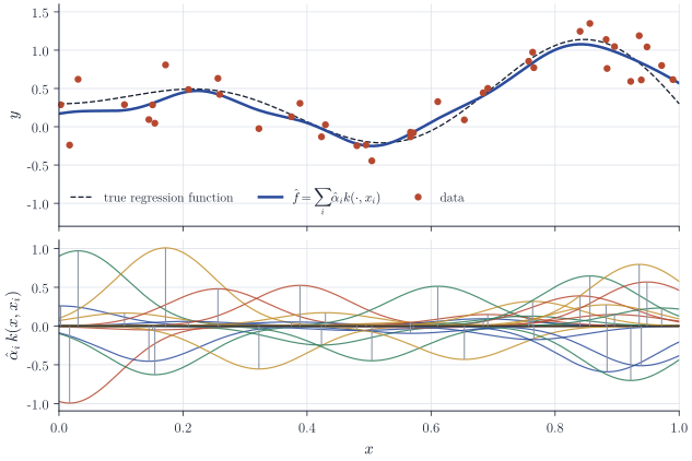
\[\Bigl\lVert \sum_{i=1}^n c_i k_{x_i} \Bigr\rVert_{\mathcal H}^2 = c^\top K c, \qquad K_{ij} = k(x_i, x_j).\]For a Gaussian kernel \(k(x,x') = \exp\{-(x-x')^2/(2w^2)\}\) on \(\R\), \(\mathcal H\) is infinite-dimensional and its norm penalizes rapid oscillation; this is the kernel used in the figures, with \(w = 0.08\).
The theorem
Theorem 1 (representer theorem). Let \(x_1, \dots, x_n \in \mathcal X\), let \(L : \R^n \to (-\infty, \infty]\) be arbitrary and \(\Omega : [0, \infty) \to \R\) non-decreasing, and set
\[J(f) = L\bigl(f(x_1), \dots, f(x_n)\bigr) + \Omega\bigl(\norm{f}_{\mathcal H}\bigr), \qquad f \in \mathcal H.\]Let \(V = \operatorname{span}\{k_{x_1}, \dots, k_{x_n}\}\) and let \(f_V\) be the orthogonal projection of \(f\) onto \(V\). Then \(J(f_V) \le J(f)\) for every \(f \in \mathcal H\), with strict inequality whenever \(\Omega\) is strictly increasing, \(f \notin V\) and \(J(f) < \infty\). Consequently, if \(J\) has a minimizer it has one in \(V\), and if \(\Omega\) is strictly increasing and \(J\) is not identically \(+\infty\), every minimizer lies in \(V\).
Proof. Write \(f = f_V + f_\perp\) with \(f_\perp \perp V\). By the reproducing property, \(f(x_i) = \inner{f_V}{k_{x_i}} + \inner{f_\perp}{k_{x_i}} = f_V(x_i)\), because \(k_{x_i} \in V\). So the loss term is the same for \(f\) and \(f_V\). By Pythagoras \(\norm{f}^2 = \norm{f_V}^2 + \norm{f_\perp}^2 \ge \norm{f_V}^2\), with strict inequality if \(f_\perp \neq 0\), and the monotonicity of \(\Omega\) transfers this to the penalty term; when the common loss value is finite, a strict inequality in the penalty gives a strict inequality in \(J\).
The proof uses nothing about the loss: it may be non-convex, discontinuous, or infinite outside a constraint set, which covers least squares, logistic and hinge losses, and interpolation constraints. What it does use is that the data enter only through point evaluations at the \(x_i\), which the reproducing property turns into inner products with elements of \(V\), and that the penalty depends on \(f\) only through its norm. If the data involved other bounded linear functionals of \(f\), such as derivatives or integrals, the same argument would apply with \(V\) spanned by their Riesz representers. Existence of a minimizer is a separate question; Theorem 1 reduces it to a problem in \(n\) variables.
Kernel ridge regression
For squared loss and a quadratic penalty, the reduced problem is explicit.
Proposition 2. For \(\lambda > 0\) and \(y \in \R^n\), the functional
\[J(f) = \frac1n \sum_{i=1}^n \bigl(y_i - f(x_i)\bigr)^2 + \lambda \norm{f}_{\mathcal H}^2\]has a unique minimizer over \(\mathcal H\), namely \(\hat f = \sum_{i=1}^n \hat\alpha_i k_{x_i}\) with \(\hat\alpha = (K + n\lambda I)^{-1}y\).
Proof. By Theorem 1 it suffices to minimize over \(V\). For \(f = \sum_i \alpha_i k_{x_i}\) the vector of fitted values is \(K\alpha\) and \(\norm{f}^2 = \alpha^\top K\alpha\), so we minimize \(g(\alpha) = n^{-1}\norm{y - K\alpha}^2 + \lambda\alpha^\top K\alpha\), a convex quadratic. Its gradient is
\[\nabla g(\alpha) = \tfrac2n K\bigl( (K + n\lambda I)\alpha - y \bigr),\]which vanishes at \(\hat\alpha\). Any other zero \(\alpha\) of the gradient satisfies \(K(K + n\lambda I)(\alpha - \hat\alpha) = 0\), hence \(K(\alpha - \hat\alpha) = 0\) because \(K\) and \(K + n\lambda I\) commute and the latter is invertible; then \(\norm{\sum_i(\alpha_i - \hat\alpha_i)k_{x_i}}^2 = (\alpha-\hat\alpha)^\top K(\alpha - \hat\alpha) = 0\), so both give the same function. Uniqueness over all of \(\mathcal H\) follows from the strict convexity of \(f \mapsto \lambda\norm{f}^2\), the loss term being convex.
The fitted function is a weighted sum of \(n\) bumps centred at the inputs. Figure 1 shows the decomposition: the weights \(\hat\alpha_i\) are not the residuals or the responses but the solution of a linear system that couples neighbouring observations, and they alternate in sign where the fit must bend.
The primal–dual identity
For the linear kernel \(k(x, x') = x^\top x'\) on \(\R^p\), \(\mathcal H\) is the space of linear functions \(x \mapsto \beta^\top x\) with \(\norm{f}_{\mathcal H} = \norm{\beta}\), and kernel ridge regression is ordinary ridge regression. With design matrix \(\mathbf X \in \R^{n\times p}\), the familiar primal solution and the representer solution must coincide:
\[\hat\beta = (\mathbf X^\top\mathbf X + n\lambda I_p)^{-1}\mathbf X^\top y = \mathbf X^\top(\mathbf X\mathbf X^\top + n\lambda I_n)^{-1} y .\]The second equality can also be checked directly: \(\mathbf X^\top(\mathbf X\mathbf X^\top + n\lambda I_n) = (\mathbf X^\top\mathbf X + n\lambda I_p)\mathbf X^\top\), and both bracketed matrices are invertible. The primal form costs \(O(np^2 + p^3)\) and the dual form \(O(n^2p + n^3)\), so the dual is preferable when \(p > n\). For a general kernel the dual form is the only one available, since the corresponding feature space may be infinite-dimensional; the representer theorem is what makes ridge regression in that space computable.
Choosing the penalty by leave-one-out
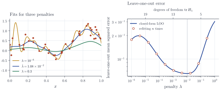
Write \(H_\lambda = K(K + n\lambda I)^{-1}\) for the matrix mapping \(y\) to the fitted values \(\hat y = K\hat\alpha\). If \(K = U\diag(\mu_j)U^\top\), then \(H_\lambda = U\diag\bigl(\mu_j/(\mu_j + n\lambda)\bigr)U^\top\), so its eigenvalues lie in \([0, 1)\), and \(\tr H_\lambda = \sum_j \mu_j/(\mu_j + n\lambda)\) serves as the effective degrees of freedom of the fit. Leave-one-out cross-validation needs no refitting.
Proposition 3. Let \(\hat f^{(-i)}\) minimize \(\sum_{j\neq i}(y_j - f(x_j))^2 + n\lambda\norm{f}^2\), the kernel ridge objective with observation \(i\) removed and the penalty weight unchanged. Then
\[y_i - \hat f^{(-i)}(x_i) = \frac{y_i - \hat y_i}{1 - (H_\lambda)_{ii}} .\]Proof. Let \(\tilde y\) equal \(y\) except that \(\tilde y_i = \hat f^{(-i)}(x_i)\). For every \(f \in \mathcal H\),
\[\begin{aligned} \sum_{j}(\tilde y_j - f(x_j))^2 + n\lambda\norm{f}^2 &\ge \sum_{j\ne i}(y_j - f(x_j))^2 + n\lambda\norm{f}^2 \\ &\ge \sum_{j\ne i}\bigl(y_j - \hat f^{(-i)}(x_j)\bigr)^2 + n\lambda\norm{\hat f^{(-i)}}^2, \end{aligned}\]and the right-hand side equals the left-hand side at \(f = \hat f^{(-i)}\), whose \(i\)-th residual for \(\tilde y\) is zero. So \(\hat f^{(-i)}\) is the full-data fit for responses \(\tilde y\), and by Proposition 2 its fitted values are \(H_\lambda\tilde y\). Reading off coordinate \(i\), \(\hat f^{(-i)}(x_i) = \sum_{j\neq i}(H_\lambda)_{ij}y_j + (H_\lambda)_{ii}\hat f^{(-i)}(x_i) = \hat y_i - (H_\lambda)_{ii}y_i + (H_\lambda)_{ii}\hat f^{(-i)}(x_i)\). Solving for \(\hat f^{(-i)}(x_i)\), which is possible because \((H_\lambda)_{ii} \le \max_j \mu_j/(\mu_j + n\lambda) < 1\), and subtracting from \(y_i\) gives the formula.
The leave-one-out error \(n^{-1}\sum_i (y_i - \hat f^{(-i)}(x_i))^2\) thus costs one eigendecomposition of \(K\) for the whole path of \(\lambda\). Figure 2 compares it with brute-force refitting and shows the usual trade-off: small \(\lambda\) interpolates the noise, large \(\lambda\) shrinks the fit towards zero.
Remarks
The kernel ridge regression estimator coincides with the posterior mean of a Gaussian process regression with covariance \(k\) and noise variance \(n\lambda\), which is why the two literatures share their formulas. Statistical guarantees for the estimator depend on how well the regression function can be approximated in \(\mathcal H\) and on the eigenvalue decay of the kernel integral operator; Caponnetto and De Vito, Optimal rates for the regularized least-squares algorithm (Foundations of Computational Mathematics, 2007), give minimax rates under such conditions. The representer theorem itself is purely algebraic and makes no probabilistic assumption, but it relies on the penalty being a non-decreasing function of the Hilbert norm. Penalties that are not of this form, such as a sparsity penalty on the coefficients of an expansion in a fixed dictionary, fall outside its scope.