How many labelings can a classifier family produce? VC dimension and the Sauer–Shelah lemma

October 12, 2026Machine learning

Empirical risk minimization chooses, from a class \(\mathcal H\) of classifiers, one that makes the fewest mistakes on the training sample. Whether this is a sensible procedure depends on whether the training error is close to the true error simultaneously for all members of \(\mathcal H\), since the minimizer is selected by looking at the data. For a finite class, Hoeffding’s inequality and a union bound over \(\abs{\mathcal H}\) classifiers settle the question. Most useful classes are infinite, but on a finite sample an infinite class acts like a finite one: it can only produce finitely many patterns of labels. The Vapnik–Chervonenkis dimension measures how fast that number of patterns grows with the sample size.

Shattering and the growth function

Let \(\mathcal H\) be a set of functions \(h : \mathcal X \to \{0, 1\}\). For a finite set \(C = \{x_1, \dots, x_n\} \subseteq \mathcal X\), the restriction of \(\mathcal H\) to \(C\) is the set of label vectors it realizes,

\[\mathcal H_C = \bigl\{ (h(x_1), \dots, h(x_n)) : h \in \mathcal H \bigr\} \subseteq \{0, 1\}^n .\]

The class shatters \(C\) if \(\mathcal H_C = \{0, 1\}^n\), that is, if every labeling of \(C\) is realized by some member of the class. The growth function is \(\Pi_{\mathcal H}(n) = \max\{\abs{\mathcal H_C} : C \subseteq \mathcal X, \abs{C} = n\}\), and the VC dimension is

\[\mathrm{VC}(\mathcal H) = \max\{ n : \Pi_{\mathcal H}(n) = 2^n \},\]

the size of the largest shattered set, or \(+\infty\) if arbitrarily large sets are shattered. The definition is asymmetric in a way that matters for proofs. To show \(\mathrm{VC}(\mathcal H) \ge d\) it suffices to exhibit one shattered set of size \(d\); to show \(\mathrm{VC}(\mathcal H) < d + 1\) one must show that no set of size \(d + 1\) is shattered.

Examples on the line

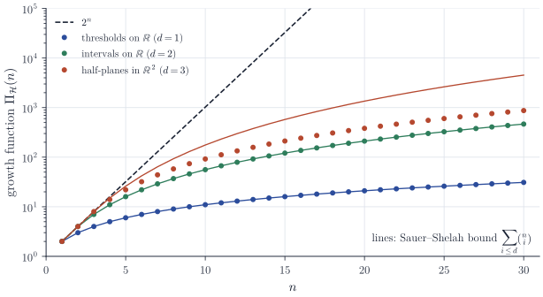
Thresholds. Let \(h_t(x) = \mathbf 1\{x \ge t\}\), \(t \in \R\). A single point receives either label, so \(\mathrm{VC} \ge 1\). For two points \(x_1 < x_2\), the labeling \((1, 0)\) would require \(x_1 \ge t > x_2\), which is impossible, so \(\mathrm{VC} = 1\). On \(n\) distinct sorted points the realized labelings are exactly those of the form \((0, \dots, 0, 1, \dots, 1)\), so \(\Pi(n) = n + 1\).

Intervals. Let \(h_{a,b}(x) = \mathbf 1\{a \le x \le b\}\). Two points can be labeled arbitrarily, but for \(x_1 < x_2 < x_3\) the labeling \((1, 0, 1)\) is impossible, because an interval containing \(x_1\) and \(x_3\) contains \(x_2\). Hence \(\mathrm{VC} = 2\). On \(n\) sorted points the positive points must form a block of consecutive points, possibly empty, so \(\Pi(n) = \binom{n}{2} + n + 1\) (choose the first and last point of a nonempty block, or a single point, or nothing).

One parameter, infinite dimension. The number of parameters is not the VC dimension. Let \(h_\omega(x) = \mathbf 1\{\sin(\omega x) > 0\}\), \(\omega > 0\), and take \(x_j = 10^{-j}\), \(j = 1, \dots, n\). Given labels \(y \in \{0,1\}^n\), put \(\omega = \pi\bigl(1 + \sum_{i=1}^n (1 - y_i) 10^i\bigr)\). Then

\[\omega x_j = \pi(1 - y_j) + \pi \Bigl( 10^{-j} + \sum_{i < j} (1 - y_i) 10^{i - j} \Bigr) + \pi \sum_{i > j} (1 - y_i) 10^{i - j} .\]

The last sum is an even multiple of \(\pi\), since \(10^{i-j}\) is even for \(i > j\). The middle term lies in \((0, \pi/9]\), since \(10^{-j} + \sum_{i<j} 10^{i-j} \le \sum_{k \ge 1} 10^{-k} = 1/9\). So modulo \(2\pi\) the angle lies in \((0, \pi/9]\) if \(y_j = 1\) and in \((\pi, 10\pi/9]\) if \(y_j = 0\), and \(h_\omega(x_j) = y_j\). Every finite set of this form is shattered, so \(\mathrm{VC} = \infty\) for a family indexed by a single real number.

Half-spaces

Let \(\mathcal H_d\) be the affine half-spaces in \(\R^d\), \(h_{w,b}(x) = \mathbf 1\{w^\top x + b > 0\}\) with \(w \in \R^d\), \(b \in \R\).

Proposition 1. \(\mathrm{VC}(\mathcal H_d) = d + 1\).

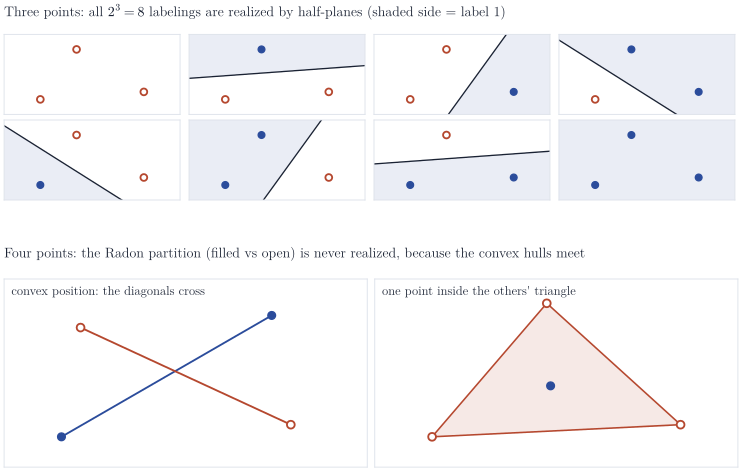
Proof. Lower bound. The points \(0, e_1, \dots, e_d\) are shattered. Given labels \(y_0, y_1, \dots, y_d \in \{0,1\}\), write \(s_i = 2y_i - 1 \in \{-1, 1\}\) and take \(b = s_0/2\) and \(w_i = s_i - b\). Then \(w^\top 0 + b = s_0/2\) and \(w^\top e_i + b = s_i\), which have the signs required.

Upper bound. Let \(x_1, \dots, x_{d+2} \in \R^d\). The \(d + 2\) vectors \((x_i, 1) \in \R^{d+1}\) are linearly dependent, so there are coefficients \(a_i\), not all zero, with \(\sum_i a_i x_i = 0\) and \(\sum_i a_i = 0\). Let \(I = \{i : a_i > 0\}\) and \(J = \{i : a_i \le 0\}\). Both are nonempty, because the \(a_i\) sum to zero and are not all zero, and \(A = \sum_{i \in I} a_i = \sum_{j \in J} (-a_j) > 0\). The point

\[z = \sum_{i \in I} \frac{a_i}{A} x_i = \sum_{j \in J} \frac{-a_j}{A} x_j\]

is a convex combination of the points in \(I\) and also of the points in \(J\) (Radon’s theorem). If some half-space labeled the points in \(I\) with \(1\) and those in \(J\) with \(0\), then \(w^\top x_i + b > 0\) for \(i \in I\) would give \(w^\top z + b > 0\) by convexity, while \(w^\top x_j + b \le 0\) for \(j \in J\) would give \(w^\top z + b \le 0\), a contradiction. So no set of \(d + 2\) points is shattered.

Figure 1. Half-planes in $\mathbb{R}^2$ ($d = 2$). Top: three points in general position are shattered. Bottom: for any four points, the partition from the proof of Proposition 1 has intersecting convex hulls. For four points in general position two cases occur, according to whether the points are in convex position (the two diagonals cross) or one point lies in the triangle of the others.

The Sauer–Shelah lemma

For \(n \le \mathrm{VC}(\mathcal H)\) the growth function equals \(2^n\). The lemma says that past the VC dimension it is at most polynomial in \(n\). The cleanest proof establishes a stronger statement: a set of labelings is no larger than the number of subsets it shatters.

Lemma 2. Let \(C\) be a finite set and \(\mathcal F \subseteq \{0, 1\}^C\). Then \(\abs{\mathcal F} \le \abs{\{S \subseteq C : \mathcal F \text{ shatters } S\}}\), where \(\mathcal F\) shatters \(S\) if every labeling of \(S\) is the restriction of some \(f \in \mathcal F\).

Proof. Induction on \(\abs{C}\). If \(C = \emptyset\), then \(\abs{\mathcal F} \le 1\), and the empty set is shattered exactly when \(\mathcal F\) is nonempty.

For \(\abs{C} \ge 1\) fix \(x \in C\) and let \(C' = C \setminus \{x\}\). Define two families of labelings of \(C'\):

\[\mathcal F_0 = \{ f\vert_{C'} : f \in \mathcal F \}, \qquad \mathcal F_1 = \{ g \in \{0,1\}^{C'} : \text{both extensions of } g \text{ to } C \text{ belong to } \mathcal F \}.\]

Each \(g \in \mathcal F_0\) has one or two extensions in \(\mathcal F\), and it has two exactly when \(g \in \mathcal F_1\), so \(\abs{\mathcal F} = \abs{\mathcal F_0} + \abs{\mathcal F_1}\). By the induction hypothesis, \(\abs{\mathcal F_0}\) is at most the number of subsets \(S \subseteq C'\) shattered by \(\mathcal F_0\), and each such \(S\) is shattered by \(\mathcal F\). Likewise \(\abs{\mathcal F_1}\) is at most the number of \(S \subseteq C'\) shattered by \(\mathcal F_1\), and for each such \(S\) the set \(S \cup \{x\}\) is shattered by \(\mathcal F\), because every labeling of \(S\) comes from some \(g \in \mathcal F_1\) and both values at \(x\) are available. The first collection consists of sets not containing \(x\) and the second of sets containing \(x\), so together they are distinct subsets of \(C\) shattered by \(\mathcal F\).

Theorem 3 (Sauer–Shelah). If \(\mathrm{VC}(\mathcal H) = d < \infty\), then for all \(n\)

\[\Pi_{\mathcal H}(n) \le \sum_{i=0}^{d} \binom{n}{i}, \qquad\text{and}\qquad \Pi_{\mathcal H}(n) \le \Bigl(\frac{en}{d}\Bigr)^d \quad (n \ge d \ge 1).\]

Proof. Apply Lemma 2 to \(\mathcal F = \mathcal H_C\) with \(\abs{C} = n\). Every subset of \(C\) shattered by \(\mathcal H_C\) is shattered by \(\mathcal H\) and so has at most \(d\) elements, and there are \(\sum_{i \le d} \binom{n}{i}\) such subsets. For the second bound, since \(d/n \le 1\),

\[\Bigl(\frac{d}{n}\Bigr)^d \sum_{i=0}^{d} \binom{n}{i} \le \sum_{i=0}^{d} \binom{n}{i} \Bigl(\frac{d}{n}\Bigr)^i \le \sum_{i=0}^{n} \binom{n}{i} \Bigl(\frac{d}{n}\Bigr)^i = \Bigl(1 + \frac{d}{n}\Bigr)^n \le e^d ,\]

and multiplying by \((n/d)^d\) gives the second bound.

The first bound is attained by thresholds and by intervals, whose growth functions computed above equal \(\sum_{i \le 1}\binom ni\) and \(\sum_{i \le 2}\binom ni\). For half-planes in \(\R^2\), the maximal number of labelings of \(n\) points, attained when no three are collinear, is \(2\sum_{k=0}^{2}\binom{n-1}{k} = n^2 - n + 2\) by Cover’s counting theorem, below the bound \(\sum_{i \le 3}\binom ni\). Figure 2 shows the dichotomy: exponential growth up to \(n = d\), polynomial growth of degree \(d\) afterwards.

Figure 2. Growth functions (points) of thresholds ($n + 1$), intervals ($\binom{n}{2} + n + 1$) and half-planes in the plane ($n^2 - n + 2$), with VC dimensions $1$, $2$ and $3$, the Sauer–Shelah bounds (lines in the same colours) and $2^n$ (dashed), on a logarithmic scale. For thresholds and intervals the bound is attained.

Why the count matters

Let \((X_1, Y_1), \dots, (X_n, Y_n)\) be i.i.d., and write \(R(h) = \P(h(X) \ne Y)\) and \(\hat R_n(h) = n^{-1}\sum_i \mathbf 1\{h(X_i) \ne Y_i\}\). If \(\hat h\) minimizes \(\hat R_n\) over \(\mathcal H\) and \(h^\circ \in \mathcal H\) is arbitrary, then

\[\begin{aligned} R(\hat h) - R(h^\circ) &= \bigl(R(\hat h) - \hat R_n(\hat h)\bigr) + \bigl(\hat R_n(\hat h) - \hat R_n(h^\circ)\bigr) + \bigl(\hat R_n(h^\circ) - R(h^\circ)\bigr) \\ &\le 2 \sup_{h \in \mathcal H} \abs{\hat R_n(h) - R(h)}, \end{aligned}\]

since the middle term is nonpositive. Everything therefore rests on the uniform deviation. The Vapnik–Chervonenkis inequality bounds it by

\[\P\Bigl( \sup_{h \in \mathcal H} \abs{\hat R_n(h) - R(h)} > \varepsilon \Bigr) \le c_1\, \Pi_{\mathcal H}(2n)\, e^{-c_2 n \varepsilon^2}\]

for absolute constants \(c_1, c_2\) (measurability conditions on \(\mathcal H\) aside). The proof replaces \(R(h)\) by the error on an independent “ghost” sample of size \(n\), which turns the supremum over \(\mathcal H\) into a maximum over the at most \(\Pi_{\mathcal H}(2n)\) distinct labelings of the \(2n\) points, and then, conditionally on the \(2n\) points, combines a union bound over these labelings with Hoeffding’s inequality for random swaps of observations between the two samples. The growth function plays exactly the role that \(\abs{\mathcal H}\) plays for a finite class. With Theorem 3 the right-hand side is at most \(c_1 (2en/d)^d e^{-c_2 n\varepsilon^2}\), which is small once \(n\varepsilon^2 \gg d \log n\), so the uniform deviation is of order \(\sqrt{d \log n / n}\) in probability. If instead \(\Pi_{\mathcal H}(n) = 2^n\) for every \(n\), the bound is useless, and this is not a weakness of the method: for every sample size there are distributions on a shattered set under which no learning rule does well.

Remarks

The VC dimension of a class with \(k\) real parameters is often of order \(k\), as for half-spaces, but the sine example shows that smoothness and parameter count alone do not control it; the classes used in practice owe their finite VC dimension to algebraic structure, such as being defined by a bounded number of polynomial inequalities. The \(\log n\) factor in the rate can be removed by chaining arguments, and the qualitative statement, that a class is learnable in the distribution-free sense if and only if its VC dimension is finite, is the content of the theorem of Blumer, Ehrenfeucht, Haussler and Warmuth.

References: V. N. Vapnik and A. Ya. Chervonenkis, “On the uniform convergence of relative frequencies of events to their probabilities”, Theory of Probability and Its Applications (1971); N. Sauer, “On the density of families of sets”, Journal of Combinatorial Theory, Series A (1972); S. Shelah, “A combinatorial problem; stability and order for models and theories in infinitary languages”, Pacific Journal of Mathematics (1972); T. M. Cover, “Geometrical and statistical properties of systems of linear inequalities with applications in pattern recognition”, IEEE Transactions on Electronic Computers (1965); A. Blumer, A. Ehrenfeucht, D. Haussler and M. K. Warmuth, “Learnability and the Vapnik–Chervonenkis dimension”, Journal of the ACM (1989). Textbook accounts are in Devroye, Györfi and Lugosi, A Probabilistic Theory of Pattern Recognition, and Shalev-Shwartz and Ben-David, Understanding Machine Learning.