Why the likelihood peaks near the truth: Wald’s consistency argument and where it breaks

Let $X_1, X_2, \dots$ be i.i.d. with density $p_{\theta_0}$ from a parametric family $\{p_\theta : \theta \in \Theta\}$. The maximum likelihood estimator maximizes $\ell_n(\theta) = \sum_{i=1}^n \log p_\theta(X_i)$. By the law of large numbers, for each fixed $\theta$,

\[\frac1n \bigl(\ell_n(\theta) - \ell_n(\theta_0)\bigr) \to \E_{\theta_0} \log \frac{p_\theta(X)}{p_{\theta_0}(X)} = -\KL(P_{\theta_0} \,\Vert\, P_\theta) \quad \text{almost surely},\]

and the limit is maximized at $\theta = \theta_0$. This is the heuristic behind consistency, and it is incomplete in an essential way: the estimator is the maximizer over all of $\Theta$ simultaneously, while the law of large numbers controls one $\theta$ at a time. A single parameter value at which the likelihood happens to be enormous is enough to ruin the estimator, even though at every fixed $\theta \neq \theta_0$ the likelihood ratio eventually loses to $\theta_0$. Wald’s 1949 argument closes the gap with compactness and one integrability condition. The argument is given below, followed by an application to a likelihood that is not concave and by three ways in which the conclusion fails.

Setting and the information inequality

Let $\{P_\theta : \theta \in \Theta\}$ be probability measures on $(\mathcal X, \mathcal A)$ with densities $p_\theta$ with respect to a $\sigma$-finite measure $\mu$, and let $X_1, X_2, \dots$ be i.i.d. $P_{\theta_0}$. Since $P_{\theta_0}(p_{\theta_0} > 0) = 1$, the log-likelihood ratio

\[m_\theta(x) = \log \frac{p_\theta(x)}{p_{\theta_0}(x)}, \qquad x \in \{p_{\theta_0} > 0\},\]

is defined almost surely, with values in $[-\infty, \infty)$. Put $M_n(\theta) = n^{-1} \sum_{i=1}^n m_\theta(X_i)$, so that maximizing $\ell_n$ is the same as maximizing $M_n$, and $M_n(\theta_0) = 0$.

Lemma 1 (information inequality). For every $\theta$, the positive part of $m_\theta(X)$ is integrable under $P_{\theta_0}$, so $\E_{\theta_0} m_\theta(X)$ is well defined in $[-\infty, \infty)$. Moreover $\E_{\theta_0} m_\theta(X) \le 0$, with equality if and only if $P_\theta = P_{\theta_0}$.

Proof. Use $\log t \le t - 1$ for $t \ge 0$ (with $\log 0 = -\infty$), with equality only at $t = 1$. With $t = p_\theta(X)/p_{\theta_0}(X)$ this gives $m_\theta(X)^+ \le t$, and

\[\E_{\theta_0} \frac{p_\theta(X)}{p_{\theta_0}(X)} = \int_{\{p_{\theta_0} > 0\}} p_\theta \, \dd\mu \le 1 ,\]

so the positive part is integrable. Taking expectations in $m_\theta(X) \le t - 1$ gives $\E_{\theta_0} m_\theta(X) \le \int_{\{p_{\theta_0} > 0\}} p_\theta \, \dd\mu - 1 \le 0$.

If equality holds, both inequalities are equalities. The first forces $t = 1$ almost surely, that is, $p_\theta = p_{\theta_0}$ $\mu$-almost everywhere on $\{p_{\theta_0} > 0\}$. The second forces $\int_{\{p_{\theta_0} = 0\}} p_\theta \, \dd\mu = 0$, so $p_\theta = 0$ $\mu$-almost everywhere on $\{p_{\theta_0} = 0\}$. Hence $p_\theta = p_{\theta_0}$ $\mu$-almost everywhere and $P_\theta = P_{\theta_0}$. The converse is immediate.

The quantity $-\E_{\theta_0} m_\theta(X)$ is the Kullback–Leibler divergence $\KL(P_{\theta_0} \Vert P_\theta)$. Under identifiability, meaning $P_\theta \ne P_{\theta_0}$ for $\theta \ne \theta_0$, Lemma 1 says that $\theta_0$ is the unique maximizer of $\theta \mapsto \E_{\theta_0} m_\theta(X)$.

Wald’s theorem

The trouble with the heuristic is the supremum over $\theta$. Wald’s idea is to replace a supremum over infinitely many parameters by a maximum over finitely many neighbourhoods, each controlled by one application of the strong law to an envelope function. Two conditions make this possible: upper semicontinuity of the log-likelihood, so that envelopes over small neighbourhoods are close to the function at the centre, and integrability of those envelopes.

Theorem 2 (Wald). Assume:

$\Theta$ is a compact metric space with metric $d$, and the model is identifiable;
for $P_{\theta_0}$-almost every $x$, the map $\theta \mapsto \log p_\theta(x)$ is upper semicontinuous on $\Theta$;
for every open ball $B \subseteq \Theta$ the map $x \mapsto \sup_{\theta' \in B} m_{\theta'}(x)$ is measurable, and every $\theta \neq \theta_0$ has an open neighbourhood $U$ with $\E_{\theta_0} \bigl[\sup_{\theta' \in U} m_{\theta'}(X)\bigr]^+ < \infty$.

Let $\hat\theta_n$ satisfy $M_n(\hat\theta_n) \ge M_n(\theta_0) = 0$ for every $n$. Then $d(\hat\theta_n, \theta_0) \to 0$ almost surely.

Proof. Step 1: a negative envelope near each $\theta \ne \theta_0$. Fix $\theta \ne \theta_0$ with neighbourhood $U$ from condition 3, and let $B_k$ be the open ball of radius $1/k$ about $\theta$. For $k \ge k_0$ we have $B_k \subseteq U$; put $f_k(x) = \sup_{\theta' \in B_k} m_{\theta'}(x)$. The sequence $f_k$ is nonincreasing in $k$ and $f_k \ge m_\theta$. Upper semicontinuity at $\theta$ means that for every $c > m_\theta(x)$ there is a ball around $\theta$ on which $m_{\theta'}(x) < c$, so $f_k(x) \downarrow m_\theta(x)$ for almost every $x$. Since $f_{k_0}^+$ is integrable, the monotone convergence theorem for nonincreasing sequences gives $\E_{\theta_0} f_k(X) \downarrow \E_{\theta_0} m_\theta(X)$, and the limit is strictly negative by Lemma 1 and identifiability (it may be $-\infty$). Choose $k$ with $\E_{\theta_0} f_k(X) < 0$ and call $U_\theta = B_k$ and $f^{\theta} = f_k$.

Step 2: compactness. Fix $\varepsilon > 0$. The set $K_\varepsilon = \{\theta : d(\theta, \theta_0) \ge \varepsilon\}$ is closed in a compact space, hence compact, and it is covered by the open sets $U_\theta$, $\theta \in K_\varepsilon$. Extract a finite subcover $U_{\theta_1}, \dots, U_{\theta_J}$. Then

\[\sup_{\theta \in K_\varepsilon} M_n(\theta) \le \max_{1 \le j \le J} \frac1n \sum_{i=1}^n f^{\theta_j}(X_i).\]

For each $j$ the strong law gives $n^{-1}\sum_i f^{\theta_j}(X_i) \to \E_{\theta_0} f^{\theta_j}(X) < 0$ almost surely. (The strong law holds for i.i.d. variables whose positive part is integrable, including the case where the mean is $-\infty$; apply it to $\max(f^{\theta_j}, -L)$ and let $L \to \infty$.) With finitely many $j$, there is an event of probability one on which $\sup_{K_\varepsilon} M_n < 0$ for all large $n$. Since $M_n(\hat\theta_n) \ge 0$, on this event $\hat\theta_n \notin K_\varepsilon$ for all large $n$. Intersecting these events over $\varepsilon = 1, 1/2, 1/3, \dots$ gives $d(\hat\theta_n, \theta_0) \to 0$ almost surely.

Several features of the statement deserve comment. No condition is imposed near $\theta_0$ itself, and no differentiability or concavity is required. The estimator need not be measurable, unique or an exact maximizer; it need only beat $\theta_0$, and the proof works verbatim if $M_n(\hat\theta_n) \ge -\varepsilon_n$ with $\varepsilon_n \to 0$. Existence is also free under the assumptions: off a null set, $M_n$ is a finite sum of upper semicontinuous functions with values in $[-\infty, \infty)$, hence upper semicontinuous on a compact set, so it attains its supremum, which is at least $M_n(\theta_0) = 0$.

Compactness is often obtained by compactifying. If $\Theta$ is not compact, one adjoins limit points, defines $p_\theta$ at the new points as a limit (allowed to be a subprobability density or zero), and checks conditions 2 and 3 there. The theorem then shows that $\hat\theta_n$ eventually stays away from the added points.

A likelihood with several local maxima

The Cauchy location family $p_\theta(x) = \pi^{-1} (1 + (x - \theta)^2)^{-1}$, $\theta \in \R$, is a standard example of a log-likelihood that is not concave: $\ell_n$ can have several local maxima, so consistency cannot be read off from a convexity argument or from a unique root of the score equation. Wald’s theorem applies directly. Compactify $\R$ to $[-\infty, \infty]$ and set $p_{\pm\infty} \equiv 0$. Since $\log p_\theta(x) \to -\infty$ as $\theta \to \pm \infty$, the map $\theta \mapsto \log p_\theta(x)$ is continuous into $[-\infty, \infty)$ on the extended line, which gives condition 2; by the same continuity, the supremum over an open ball equals the supremum over the rational points in it, which settles the measurability requirement in condition 3. For condition 3, a single envelope works for every neighbourhood: after translating to $\theta_0 = 0$ without loss of generality,

\[m_\theta(x) = \log(1 + x^2) - \log\bigl(1 + (x - \theta)^2\bigr) \le \log(1 + x^2),\]

and $\E_0 \log(1 + X^2) = 2 \log 2 < \infty$. Identifiability is clear for finite $\theta$, and at the two added points $m_{\pm\infty} \equiv -\infty$, so $\E_0 m_{\pm\infty}(X) < 0$, which is all that Step 1 uses. (A metric on the extended line is $d(s, t) = \abs{\arctan s - \arctan t}$.) Hence every global maximizer of the Cauchy likelihood converges to $\theta_0$ almost surely. The limit criterion has the closed form $\E_0 m_\theta(X) = -\log(1 + \theta^2/4)$.

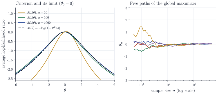
Left: average log-likelihood ratio curves for the Cauchy location model at three sample sizes, approaching the limit curve. Right: five paths of the maximum likelihood estimate against sample size, converging to zero. — Figure 1. Cauchy location model with $\theta_0 = 0$. Left: $M_n(\theta)$ along one sample path for $n = 10, 100, 1000$, and the limit $M(\theta) = -\log(1 + \theta^2/4)$. Right: the global maximizer $\hat\theta_n$ (found by a grid search on $[-15, 15]$ followed by local refinement) along five independent paths.

In the left panel the curves $M_n$ approach $M$, whose gap $M(0) - M(\theta) \ge \log(1 + \varepsilon^2/4)$ for $\abs{\theta} \ge \varepsilon$ keeps every such $\theta$ from competing with $\theta_0$ once $n$ is large. The proof needs less than uniform convergence of $M_n$ to $M$: only an upper bound for $M_n$ off a neighbourhood of $\theta_0$, supplied by finitely many envelope averages.

Where the argument breaks

Unbounded likelihoods. Consider the mixture $\tfrac12 N(0, 1) + \tfrac12 N(\mu, \sigma^2)$ with $\theta = (\mu, \sigma) \in \R \times (0, \infty)$. Setting $\mu = Y_1$, the first observation, and keeping only the second component in the first factor,

\[\ell_n(Y_1, \sigma) \ge \log \frac{1}{2\sqrt{2\pi}\,\sigma} + \sum_{i=2}^n \log \Bigl(\tfrac12 \phi(Y_i)\Bigr) \to \infty \qquad (\sigma \downarrow 0),\]

where $\phi$ is the standard normal density. The likelihood has no maximizer, and every $\hat\theta_n$ with $M_n(\hat\theta_n) \ge 0$ can be chosen with $\sigma$ arbitrarily small. In terms of Theorem 2, compactifying the scale at $\sigma = 0$ produces boundary points $(\mu, 0)$. Every neighbourhood of such a point contains the parameters $(x, \sigma')$, $\sigma'$ small, for all $x$ in an interval around $\mu$, so the envelope in condition 3 equals $+\infty$ on a set of positive probability.

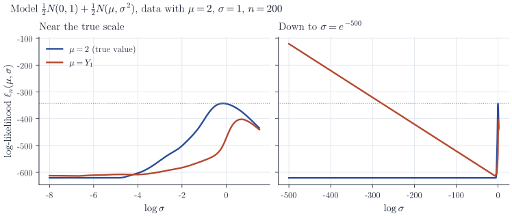
Log-likelihood of a two-component normal mixture against log sigma, at the true mean and at mu equal to the first observation; the latter grows without bound as sigma tends to zero. — Figure 2. Log-likelihood of $\frac12 N(0,1) + \frac12 N(\mu, \sigma^2)$ for one sample of size $200$ from $\mu = 2$, $\sigma = 1$, as a function of $\log\sigma$. Left: near the true scale, where the curve for $\mu = 2$ has a well-defined local maximum (dotted line). Right: the same curves down to $\sigma = e^{-500}$. With $\mu = Y_1$ the log-likelihood grows linearly in $-\log\sigma$ and exceeds that local maximum once $\log\sigma$ is below about $-278$.

The degeneracy is real but numerically remote, which is why local optimizers such as EM usually return the sensible local maximum. Two standard repairs restore a theorem: restricting to $\sigma \ge c > 0$, after which Wald’s conditions can be checked on the constrained space, or proving consistency of a suitably chosen local maximizer, which requires the differentiability conditions of Cramér-type theory.

Growing numbers of parameters. In the Neyman–Scott problem one observes pairs $X_{i1}, X_{i2} \sim N(\mu_i, \sigma^2)$, independent, $i = 1, \dots, n$. Each pair brings its own nuisance mean. The maximum likelihood estimators are $\hat\mu_i = (X_{i1} + X_{i2})/2$ and

\[\hat\sigma^2_n = \frac{1}{2n} \sum_{i=1}^n \sum_{j=1}^2 (X_{ij} - \hat\mu_i)^2 = \frac{1}{4n} \sum_{i=1}^n (X_{i1} - X_{i2})^2 \to \frac{\sigma^2}{2} \quad \text{almost surely},\]

because $X_{i1} - X_{i2} \sim N(0, 2\sigma^2)$ are i.i.d. and the strong law applies. The estimator converges, to the wrong value. The data are not i.i.d. from a fixed finite-dimensional model, so Theorem 2 has nothing to say; each $\mu_i$ is estimated from two observations and the resulting error is never averaged away.

Failure of the envelope condition alone. Identifiability, compactness and continuity are not enough by themselves. Ferguson (1982) constructed a family indexed by $\theta \in [0, 1]$, continuous in $\theta$ and identifiable, for which the maximum likelihood estimator exists and converges almost surely to $1$ whatever the true value. The densities develop increasingly tall and narrow spikes as $\theta \to 1$, so the integrability in condition 3 fails near $\theta = 1$, in the same way it fails at the boundary in the mixture example.

Remarks

Theorem 2 delivers strong consistency, which is more than the convergence in probability usually needed. The conditions concern the model and the true parameter only through integrability under $P_{\theta_0}$. When the data are not generated by any member of the model, the same proof with $m_\theta = \log(p_\theta/p_{\theta^*})$ shows convergence to the minimizer $\theta^*$ of $\KL(P \Vert P_\theta)$, provided that minimizer is unique and the corresponding envelope conditions hold under the true law $P$.

The original source is A. Wald, “Note on the consistency of the maximum likelihood estimate”, Annals of Mathematical Statistics (1949). Textbook treatments are in Chapter 5 of van der Vaart, Asymptotic Statistics, and in Ferguson, A Course in Large Sample Theory. The counterexamples are from J. Neyman and E. L. Scott, “Consistent estimates based on partially consistent observations”, Econometrica (1948), and T. S. Ferguson, “An inconsistent maximum likelihood estimate”, Journal of the American Statistical Association (1982).