The expectation–maximization algorithm

Many statistical models are easiest to write down with variables that are not observed: the component labels in a mixture model, the hidden states of a hidden Markov model, the missing entries of an incomplete data set. If those variables were observed, the likelihood would often be simple to maximize. The expectation–maximization (EM) algorithm of Dempster, Laird and Rubin (1977) exploits this. It maximizes the likelihood of the observed data by repeatedly maximizing the expected complete-data log-likelihood, where the expectation is over the unobserved variables given the data and the current parameter value.

I was led back to EM while working on Poisson mixtures for count data, which also serve as the running example below.

Setting

Let $x$ be the observed data, $z$ the latent variables, and $\theta \in \Theta$ the parameter. The model specifies a complete-data density $p(x, z \mid \theta)$. To keep the notation light, $z$ is taken to be discrete; for continuous $z$, sums become integrals. The quantity we want to maximize is the observed-data log-likelihood

\[\ell(\theta) = \log p(x \mid \theta) = \log \sum_{z} p(x, z \mid \theta).\]

The logarithm sits outside the sum, and this is where the difficulty lies. Consider a mixture of $K$ densities $f(\cdot \mid \lambda_k)$ with weights $\pi_k$, observed through an i.i.d. sample $x_1, \dots, x_n$, and let $z_i \in \{1, \dots, K\}$ be the label of the component that generated $x_i$. Because the pairs $(x_i, z_i)$ are independent, the sum over the $K^n$ label configurations factorizes and

\[\ell(\theta) = \sum_{i=1}^n \log \sum_{k=1}^K \pi_k f(x_i \mid \lambda_k),\]

which costs only $nK$ terms to evaluate. The problem is not evaluation but maximization: the log of a sum couples all the parameters, and setting the gradient to zero gives equations with no closed-form solution. The complete-data log-likelihood, in contrast,

\[\log p(x, z \mid \theta) = \sum_{i=1}^n \sum_{k=1}^K \mathbf 1\{z_i = k\} \bigl\{\log \pi_k + \log f(x_i \mid \lambda_k)\bigr\},\]

separates into a term for the weights and one term for each component, and for many families $f$ each piece is maximized in closed form. EM transfers this simplicity to the observed-data problem.

A lower bound on the log-likelihood

Let $q$ be any probability mass function on the values of $z$, and define

\[F(q, \theta) = \sum_z q(z) \log \frac{p(x, z \mid \theta)}{q(z)} = \E_q\bigl[\log p(x, Z \mid \theta)\bigr] + H(q),\]

where $H(q) = -\sum_z q(z) \log q(z)$ is the entropy of $q$. Writing $p(x, z \mid \theta) = p(z \mid x, \theta)\, p(x \mid \theta)$ gives, whenever $p(x \mid \theta) > 0$ and $F(q, \theta)$ is finite,

\[\ell(\theta) = F(q, \theta) + \KL\bigl(q \,\Vert\, p(\cdot \mid x, \theta)\bigr).\]

Since the Kullback–Leibler divergence is nonnegative and vanishes only when its arguments coincide, $F(q, \theta) \le \ell(\theta)$ for all $q$, with equality if and only if $q = p(\cdot \mid x, \theta)$. This is the same identity that underlies variational inference, with the evidence replaced by the likelihood at a fixed $\theta$; the proof is given in the note on variational inference. The functional $F$ is a lower bound on $\ell$ that touches it when $q$ is the conditional distribution of the latent variables.

The algorithm

Starting from $\theta_0$, EM alternates two steps.

E-step. Compute the conditional distribution $p(z \mid x, \theta_t)$ and the function
\[Q(\theta \mid \theta_t) = \E\bigl[\log p(x, Z \mid \theta) \,\big\vert\, x, \theta_t\bigr] = \sum_z p(z \mid x, \theta_t) \log p(x, z \mid \theta).\]
M-step. Set $\theta_{t+1} \in \argmax_{\theta \in \Theta} Q(\theta \mid \theta_t)$.

In terms of $F$, the E-step maximizes $F(q, \theta_t)$ over $q$, which gives $q_{t+1} = p(\cdot \mid x, \theta_t)$ and makes the bound tight at $\theta_t$. The M-step maximizes $F(q_{t+1}, \theta)$ over $\theta$, and since $F(q_{t+1}, \theta) = Q(\theta \mid \theta_t) + H(q_{t+1})$ with an entropy term that does not depend on $\theta$, this is the same as maximizing $Q(\cdot \mid \theta_t)$. EM is coordinate ascent on $F$.

Theorem 1 (monotonicity). If $\ell(\theta_t)$ is finite and $Q(\theta_{t+1} \mid \theta_t) \ge Q(\theta_t \mid \theta_t)$, then $\ell(\theta_{t+1}) \ge \ell(\theta_t)$.

Proof. Let $q_{t+1} = p(\cdot \mid x, \theta_t)$. The bound is tight at $\theta_t$, it lies below $\ell$ everywhere, and $F(q_{t+1}, \theta) - F(q_{t+1}, \theta_t) = Q(\theta \mid \theta_t) - Q(\theta_t \mid \theta_t)$. Hence

\[\ell(\theta_{t+1}) \ge F(q_{t+1}, \theta_{t+1}) = F(q_{t+1}, \theta_t) + Q(\theta_{t+1} \mid \theta_t) - Q(\theta_t \mid \theta_t) \ge F(q_{t+1}, \theta_t) = \ell(\theta_t).\]

The theorem only uses that the M-step does not decrease $Q$, so it covers generalized EM algorithms, which replace the full maximization by any improvement, for instance a single Newton step or a cycle of conditional maximizations.

The same argument is often written with the decomposition

\[\ell(\theta) = Q(\theta \mid \theta_t) + R(\theta \mid \theta_t), \qquad R(\theta \mid \theta_t) = -\E\bigl[\log p(Z \mid x, \theta) \,\big\vert\, x, \theta_t\bigr],\]

obtained by taking the conditional expectation of $\log p(x \mid \theta) = \log p(x, Z \mid \theta) - \log p(Z \mid x, \theta)$. The term $R(\theta \mid \theta_t)$ is the cross-entropy of $p(\cdot \mid x, \theta)$ relative to $p(\cdot \mid x, \theta_t)$. It does depend on $\theta$, but by Gibbs’ inequality it is minimized over $\theta$ at $\theta = \theta_t$, so any increase in $Q$ is an increase in $\ell$ at least as large. This decomposition also gives a useful identity. If $\theta_t$ is an interior point and both $Q(\cdot \mid \theta_t)$ and $R(\cdot \mid \theta_t)$ are differentiable there, the minimum of $R(\cdot \mid \theta_t)$ at $\theta_t$ forces its gradient to vanish, and

\[\nabla \ell(\theta_t) = \nabla_\theta Q(\theta \mid \theta_t)\big\vert_{\theta = \theta_t}.\]

The score of the observed data equals the expected complete-data score. In particular, an interior fixed point of EM, one with $\theta_t \in \argmax_\theta Q(\theta \mid \theta_t)$, is a stationary point of $\ell$.

Convergence

Monotonicity alone gives that $\ell(\theta_t)$ converges whenever $\ell$ is bounded above on the iterates, which holds for instance for any model with a discrete observation space, where $\ell \le 0$. Convergence of the parameter sequence itself is more delicate. Wu (1983) gave conditions, including continuity of $Q(\theta \mid \phi)$ in both arguments and compactness of the set $\{\theta : \ell(\theta) \ge \ell(\theta_0)\}$, under which every limit point of the EM sequence is a stationary point of $\ell$; with additional conditions, such as isolated stationary points, the sequence converges. Three caveats follow from the word “stationary”.

The limit can be a local maximum rather than the global one, which is why EM is usually run from several starting points.
The limit can be a saddle point. The example below contains one that EM reaches from a whole family of starting values.
Where the likelihood is unbounded, as for Gaussian mixtures with unequal variances when one component collapses onto a single observation, EM can be drawn towards a degenerate solution, and the maximum likelihood estimator itself must be defined with care.

Near a local maximum where the observed information is positive definite, EM converges linearly. The rate is the largest eigenvalue of the fraction of missing information, the matrix $I_c^{-1} I_m$ evaluated at the limit, in which $I_c$ is the complete-data information averaged over the conditional distribution of $z$ given $x$, $I_o$ is the observed-data information, and $I_m = I_c - I_o$ is the information lost because $z$ is unobserved. When the components of a mixture overlap heavily, most of the information about the labels is missing and EM is slow.

Example: a Poisson mixture

Let $x_1, \dots, x_n$ be i.i.d. counts from the mixture $\sum_{k=1}^K \pi_k\, \mathrm{Pois}(\lambda_k)$, with weights $\pi_k > 0$ summing to one and rates $\lambda_k > 0$. The model is identifiable up to relabelling of the components when the $\lambda_k$ are distinct: the probability generating function of the mixture is $s \mapsto \sum_k \pi_k e^{\lambda_k (s-1)}$, and exponential functions with distinct rates are linearly independent, so the function determines the pairs $(\pi_k, \lambda_k)$. With latent labels $z_i$, the complete-data log-likelihood is

\[\log p(x, z \mid \theta) = \sum_{i=1}^n \sum_{k=1}^K \mathbf 1\{z_i = k\} \bigl\{\log \pi_k + x_i \log \lambda_k - \lambda_k - \log x_i!\bigr\}.\]

E-step. Given $\theta_t$, the labels are conditionally independent with

\[r_{ik} = \P(z_i = k \mid x_i, \theta_t) = \frac{\pi_k^{(t)} \lambda_k^{(t)\, x_i} e^{-\lambda_k^{(t)}}}{\sum_{l=1}^K \pi_l^{(t)} \lambda_l^{(t)\, x_i} e^{-\lambda_l^{(t)}}},\]

the responsibility of component $k$ for observation $i$; the factor $1/x_i!$ cancels. Since the complete-data log-likelihood is linear in the indicators, the E-step only replaces $\mathbf 1\{z_i = k\}$ by $r_{ik}$:

\[Q(\theta \mid \theta_t) = \sum_{k=1}^K N_k \log \pi_k + \sum_{k=1}^K \Bigl(\log\lambda_k \sum_{i=1}^n r_{ik} x_i - N_k \lambda_k\Bigr) + \text{const}, \qquad N_k = \sum_{i=1}^n r_{ik}.\]

M-step. The weights and the rates appear in separate terms. For the weights, $\sum_k N_k \log \pi_k = n \sum_k (N_k/n)\log \pi_k$, and Gibbs’ inequality shows that this is maximized over the probability simplex by $\pi_k = N_k/n$. For each rate, the function $\lambda \mapsto \log\lambda \sum_i r_{ik} x_i - N_k\lambda$ is strictly concave on $(0, \infty)$, with derivative zero at

\[\lambda_k^{(t+1)} = \frac{\sum_{i=1}^n r_{ik} x_i}{\sum_{i=1}^n r_{ik}},\]

provided $\sum_i r_{ik} x_i > 0$. The new rate is a weighted sample mean, with each count weighted by the probability that it belongs to component $k$: the same formula as with known labels, with indicators replaced by probabilities.

import numpy as np
from scipy.special import logsumexp
from scipy.stats import poisson

def em_poisson_mixture(x, pi, lam, iters=500, tol=1e-10):
    x, pi, lam = np.asarray(x), np.asarray(pi, float), np.asarray(lam, float)
    ll_old = -np.inf
    for _ in range(iters):
        logw = np.log(pi) + poisson.logpmf(x[:, None], lam)  # n x K
        lse = logsumexp(logw, axis=1, keepdims=True)
        ll = lse.sum()                     # log-likelihood
        if ll - ll_old < tol:
            break
        ll_old = ll
        r = np.exp(logw - lse)             # E-step
        Nk = r.sum(axis=0)                 # M-step
        pi, lam = Nk / x.size, (r * x[:, None]).sum(axis=0) / Nk
    return pi, lam, ll

Working on the log scale avoids underflow of $\lambda^{x} e^{-\lambda}$ for large counts, and the log-likelihood comes for free from the normalizing constants of the E-step.

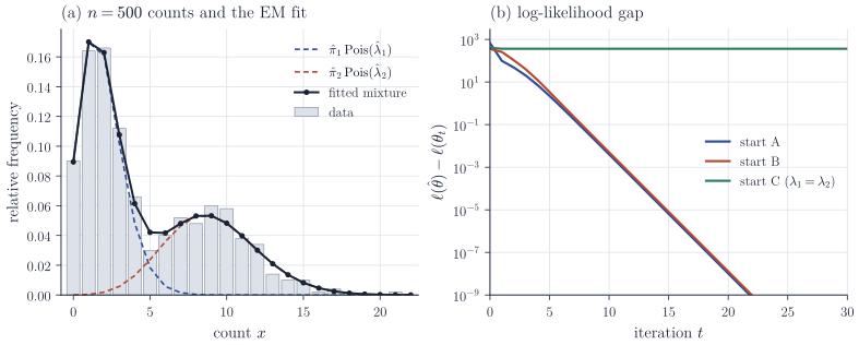
The figure shows a simulated sample of $n = 500$ counts from $0.6\,\mathrm{Pois}(2) + 0.4\,\mathrm{Pois}(9)$. EM gives $\hat\pi = (0.596, 0.404)$ and $\hat\lambda = (1.90, 9.07)$. Starts A and B reach the same maximum and the log-likelihood gap decreases geometrically, as the linear rate predicts. Start C has equal rates. Then all responsibilities equal the current weights, both rates are updated to the sample mean $\bar x = 4.79$, and the iteration stays there forever: the parameter at which the mixture collapses to a single Poisson distribution is a fixed point of EM and a stationary point of $\ell$, but not a maximum. It is a saddle point. Moving both rates together away from $\bar x$ lowers $\ell$, since $\bar x$ maximizes the one-component Poisson likelihood. Splitting them symmetrically, $\lambda = (\bar x - \delta, \bar x + \delta)$ with the weights $(0.5, 0.5)$ of start C, raises it: a second-order expansion in $\delta$ gives $\ell(\delta) - \ell(0) = \tfrac12 \delta^2 \sum_i \{(x_i - \bar x)^2 - x_i\}/\bar x^2 + O(\delta^4)$, which is positive for small $\delta$ because the sample variance of the counts exceeds their mean. Any start with equal rates ends at such a point, whatever the weights, and the remedy is to break the symmetry.

Histogram of simulated counts with fitted Poisson mixture, and log-likelihood gap along EM iterations — Figure 1. EM for a two-component Poisson mixture. (a) Relative frequencies of $n = 500$ simulated counts, the fitted mixture and its weighted components. (b) $\ell(\hat\theta) - \ell(\theta_t)$ on a log scale for three starting values: A, $\pi = (0.5, 0.5)$, $\lambda = (1, 3)$; B, $\pi = (0.9, 0.1)$, $\lambda = (5, 6)$; C, $\pi = (0.5, 0.5)$, $\lambda = (4, 4)$. From C the iteration is stuck at the one-component fit, a saddle point of the likelihood.

Because the Poisson probability mass function is at most one, $\ell \le 0$ for every parameter value, so the likelihood is bounded and the degeneracies of Gaussian mixtures cannot occur. A rate can still go to zero if a component ends up responsible only for zero counts, which corresponds to a point mass at zero, and a weight can go to zero if a component loses all its responsibility.

Remarks

When the E-step is intractable, it can be replaced by a Monte Carlo average (Monte Carlo EM, stochastic EM) or by a restricted approximation of $p(z \mid x, \theta)$, which turns EM into variational EM. When the M-step is intractable, it can be split into conditional maximizations (ECM). A Gaussian mixture example is worked out in a separate note.

The original reference is Dempster, Laird and Rubin, “Maximum likelihood from incomplete data via the EM algorithm” (Journal of the Royal Statistical Society, Series B, 1977). The convergence theory is due to Wu, “On the convergence properties of the EM algorithm” (Annals of Statistics, 1983). McLachlan and Krishnan, The EM Algorithm and Extensions, is a comprehensive treatment.