Inverse transform sampling

Most random number generators produce, at bottom, independent draws that behave like samples from the uniform distribution on $(0,1)$. Inverse transform sampling turns such a draw into a draw from any distribution on the real line: evaluate the quantile function at the uniform. The method is exact, it needs one uniform per output, and it is monotone in the uniform, which makes it the natural choice whenever samples from different distributions must be coupled. Its practical limitation is that the quantile function must be computable.

Textbook statements often assume that $F$ is continuous and strictly increasing, so that $F^{-1}$ is an ordinary inverse. That assumption excludes discrete distributions, which then get a separate algorithm and a separate proof. With the right definition of $F^{-1}$, a single argument handles every case.

The generalized inverse

Let $F$ be a distribution function: nondecreasing, right-continuous, with $F(x) \to 0$ as $x \to -\infty$ and $F(x) \to 1$ as $x \to \infty$. Its generalized inverse, or quantile function, is

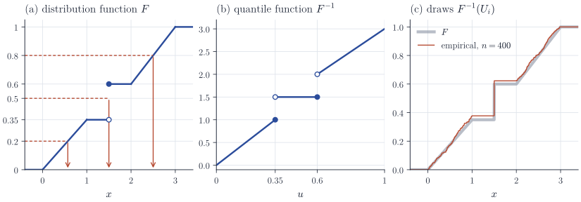
\[F^{-1}(u) = \inf\{x \in \R : F(x) \ge u\}, \qquad 0 < u < 1 .\]

For $u \in (0,1)$ the set $\{x : F(x) \ge u\}$ is nonempty because $F(x) \to 1$, and bounded below because $F(x) \to 0$, so $F^{-1}(u)$ is a real number. Where $F$ is continuous and strictly increasing, $F^{-1}$ is the ordinary inverse. Where $F$ is flat, say $F = c$ on a maximal interval $[a, b)$, $F^{-1}$ jumps at $u = c$, and $F^{-1}(c)$ is the left endpoint of the flat stretch. Where $F$ jumps, say from $F(x-) = c_1$ to $F(x) = c_2$, $F^{-1}$ is constant and equal to $x$ on $(c_1, c_2]$. Panels (a) and (b) of the figure below show both phenomena.

Everything rests on the following equivalence.

Lemma 1. For $u \in (0,1)$ and $x \in \R$,

\[F^{-1}(u) \le x \iff u \le F(x).\]

Proof. The set $S_u = \{y : F(y) \ge u\}$ is an interval unbounded to the right, because $F$ is nondecreasing. It contains its infimum $F^{-1}(u)$: if $y_k \downarrow F^{-1}(u)$ with $y_k \in S_u$, right-continuity gives $F(F^{-1}(u)) = \lim_k F(y_k) \ge u$. Hence $S_u = [F^{-1}(u), \infty)$, and $x \in S_u$, that is $u \le F(x)$, holds if and only if $x \ge F^{-1}(u)$.

Two consequences are used below. Taking $x = F^{-1}(u)$ gives $F(F^{-1}(u)) \ge u$, with equality when $F$ is continuous, by the intermediate value theorem. And $F^{-1}$ is nondecreasing on $(0,1)$, hence Borel measurable, so $F^{-1}(U)$ is a random variable whenever $U$ is.

The sampling theorem

Theorem 2. Let $U$ be uniform on $(0,1)$ and let $F$ be any distribution function. Then $X = F^{-1}(U)$ has distribution function $F$.

Proof. By Lemma 1, the events $\{F^{-1}(U) \le x\}$ and $\{U \le F(x)\}$ coincide for every $x$, so

\[\P(X \le x) = \P\bigl(U \le F(x)\bigr) = F(x),\]

since $\P(U \le t) = t$ for $t \in [0,1]$.

The algorithm is therefore: draw $U$, return $F^{-1}(U)$. Whether $U$ is taken uniform on $(0,1)$ or on $[0,1]$ is immaterial, since the endpoints have probability zero; restricting to the open interval only avoids the values $F^{-1}(0) = -\infty$ and $F^{-1}(1)$, which may be $+\infty$.

A distribution function with a flat stretch and a jump, its quantile function, and the empirical distribution of inverse-transform draws — Figure 1. The mixture $0.35\,\mathrm{Unif}(0,1) + 0.25\,\delta_{1.5} + 0.40\,\mathrm{Unif}(2,3)$. (a) Its distribution function, with $u = 0.2, 0.5, 0.8$ mapped to $F^{-1}(u)$; every $u \in (0.35, 0.6]$ is mapped to the atom at $1.5$. (b) The quantile function: the flat stretches of $F$ on $[1, 1.5)$ and $[1.5, 2)$ become jumps of $F^{-1}$, and the jump of $F$ becomes a flat stretch. Filled and open circles mark attained and omitted values. (c) The empirical distribution function of $400$ draws $F^{-1}(U_i)$ against $F$.

Continuous examples

When $F$ has an explicit inverse, the algorithm is one line.

Exponential with rate $\lambda > 0$: $F(x) = 1 - e^{-\lambda x}$ for $x \ge 0$, so $F^{-1}(u) = -\log(1-u)/\lambda$. Since $1 - U$ is again uniform, $-\log(U)/\lambda$ works equally well.
Cauchy: $F(x) = \tfrac12 + \tfrac1\pi \arctan x$, so $F^{-1}(u) = \tan\bigl(\pi(u - \tfrac12)\bigr)$.
Weibull with shape $k > 0$ and scale $s > 0$: $F(x) = 1 - \exp\{-(x/s)^k\}$ for $x \ge 0$, so $F^{-1}(u) = s\,\{-\log(1-u)\}^{1/k}$.

When no closed form exists, $F^{-1}$ can still be computed numerically, either by solving $F(x) = u$ with a root finder (bisection is safe because $F$ is monotone) or by a dedicated approximation. The normal quantile function is the standard case. It has no elementary closed form, but rational approximations accurate to roughly machine precision are available, for example Wichura’s algorithm AS 241 (Applied Statistics, 1988), which R uses in qnorm. R’s default normal generator is in fact inversion of this kind. Whether inversion is the fastest option depends on the cost of the quantile function; special-purpose methods such as the Box–Muller transform or the ziggurat algorithm are faster for the normal in many implementations.

Discrete distributions

Let $X$ take values $x_1 < x_2 < \cdots$ (finitely or countably many) with probabilities $p_k > 0$, and write $F_k = p_1 + \dots + p_k$, $F_0 = 0$. Then $F$ is a step function with $F(x_k) = F_k$, and Lemma 1 gives

\[F^{-1}(u) = x_k \iff F_{k-1} < u \le F_k .\]

So the general algorithm specializes to: draw $U$ and return $x_K$, where $K$ is the first index with $F_K \ge U$. Theorem 2 already shows this is correct, and it is also immediate, since $\P(F_{k-1} < U \le F_k) = p_k$.

Finding $K$ is a search problem. A sequential search through $F_1, F_2, \dots$ uses $K$ comparisons, so its expected cost is $\E K = \sum_k k\, p_k$; listing the values in order of decreasing probability reduces this cost. The reordered sampler is still exact, because $\P(F_{k-1} < U \le F_k) = p_k$ for any enumeration of the support, but it is no longer the monotone map $F^{-1}$. For a finite support of size $m$, binary search on the cumulative sums costs $O(\log m)$ per draw, and Walker’s alias method reduces the cost to $O(1)$ per draw after $O(m)$ preprocessing, at the price of using a different, non-monotone map from uniforms to values.

import numpy as np

def sample_discrete(values, probs, size, rng):
    """Inverse transform sampling from a finite distribution."""
    cdf = np.cumsum(probs)
    cdf[-1] = 1.0                      # guard against rounding in the last partial sum
    u = rng.random(size)               # uniform on [0, 1)
    k = np.searchsorted(cdf, u, side="left")   # first k with cdf[k] >= u
    return np.asarray(values)[k]

For some discrete families the search can be solved in closed form. For the geometric distribution on $\{1, 2, \dots\}$ with success probability $p$, $F(k) = 1 - (1-p)^k$, and the smallest integer $k$ with $1 - (1-p)^k \ge u$ is

\[F^{-1}(u) = \Bigl\lceil \frac{\log(1-u)}{\log(1-p)} \Bigr\rceil .\]

The converse: the probability integral transform

Inverse transform sampling maps uniforms to $F$. In the other direction, if $X$ has a continuous distribution function $F$, then $F(X)$ is uniform on $(0,1)$. To see this, note that Lemma 1 is equivalent to $u > F(x) \iff F^{-1}(u) > x$, so for $u \in (0,1)$

\[\P\bigl(F(X) < u\bigr) = \P\bigl(X < F^{-1}(u)\bigr) = F\bigl(F^{-1}(u)\bigr) = u ,\]

where the second equality uses continuity of $F$ (so that $\P(X < y) = F(y)$) and the third uses $F(F^{-1}(u)) = u$ for continuous $F$. Continuity is necessary: if $F$ has an atom, $F(X)$ takes some value with positive probability and cannot be uniform. This direction is the basis of p-values for continuous test statistics, of the Kolmogorov–Smirnov test’s distribution-free null distribution, and of copula models, where each margin is transformed to the uniform scale.

Practical remarks

Truncation. To sample $X$ conditionally on $a < X \le b$, where $F(a) < F(b)$, draw $V$ uniform on $(F(a), F(b))$ and return $F^{-1}(V)$. By Lemma 1, for $a \le x \le b$,

\[\P\bigl(F^{-1}(V) \le x\bigr) = \P\bigl(V \le F(x)\bigr) = \frac{F(x) - F(a)}{F(b) - F(a)},\]

which is the conditional distribution function. Unlike rejection, this costs one uniform per draw however small $F(b) - F(a)$ is. Far in the upper tail, $F(a)$ is close to one and loses relative precision in floating point; it is then better to work with the survival function $1 - F$ and its inverse, which accurate libraries provide separately.

Coupling. Because $F^{-1}$ is nondecreasing, using the same $U$ for two distributions $F$ and $G$ produces a pair $(F^{-1}(U), G^{-1}(U))$ that is as positively dependent as possible given its margins. This is what makes common random numbers effective when comparing two simulated systems, and it is also why inversion combines well with variance reduction by antithetic variables, where $U$ and $1 - U$ yield negatively correlated outputs, and with quasi-Monte Carlo point sets, whose even spread over $(0,1)$ is transferred monotonically to the target distribution.

A comprehensive reference on inversion and its alternatives is Devroye, Non-Uniform Random Variate Generation (1986).