Sampling from the multivariate normal distribution
Standard normal variables are cheap to generate: every numerical library provides them, by inversion of the normal distribution function (see the note on inverse transform sampling) or by faster special-purpose methods. A draw from a general multivariate normal distribution is obtained from independent standard normals by an affine map, and the only real decisions are which matrix factor to use and how to avoid forming inverses. Below I work through those decisions for the two common ways of specifying a Gaussian, by its covariance matrix and by its precision matrix.
One dimension
If \(z \sim N(0, 1)\), then \(x = \mu + \sigma z \sim N(\mu, \sigma^2)\), where \(\sigma > 0\) is the standard deviation: adding \(\mu\) shifts the location, and multiplying by \(\sigma\) rescales the spread, multiplying the variance by \(\sigma^2\). If the distribution is specified by its precision \(\tau = 1/\sigma^2\) instead, the same draw is \(x = \mu + \tau^{-1/2} z\). The multivariate case replaces \(\sigma\) by a matrix whose “square” is the covariance matrix, and \(\tau^{-1/2}\) by a matrix built from the precision matrix. The difference is that matrix square roots are not unique and inverses are expensive.
Affine images of standard normal vectors
A random vector \(y \in \R^d\) is multivariate normal with mean \(\mu\) and covariance \(\Sigma\), written \(y \sim N_d(\mu, \Sigma)\), if its characteristic function is
\[\E \exp(i t^\top y) = \exp\bigl(i t^\top \mu - \tfrac12 t^\top \Sigma t\bigr), \qquad t \in \R^d ,\]where \(\Sigma\) is symmetric positive semidefinite. This definition includes singular covariance matrices. When \(\Sigma\) is positive definite, \(y\) has the familiar density
\[p(y) = (2\pi)^{-d/2} (\det \Sigma)^{-1/2} \exp\Bigl\{-\tfrac12 (y - \mu)^\top \Sigma^{-1} (y - \mu)\Bigr\}.\]Proposition 1. Let \(z \sim N_k(0, I_k)\), let \(A\) be a \(d \times k\) matrix with \(AA^\top = \Sigma\), and let \(\mu \in \R^d\). Then \(y = \mu + Az \sim N_d(\mu, \Sigma)\).
Proof. The coordinates of \(z\) are independent standard normals, so \(\E\exp(i s^\top z) = \prod_{j=1}^k e^{-s_j^2/2} = \exp(-\tfrac12 \norm{s}^2)\) for \(s \in \R^k\). With \(s = A^\top t\),
\[\E \exp(i t^\top y) = e^{i t^\top \mu}\, \E \exp\bigl(i (A^\top t)^\top z\bigr) = \exp\bigl(i t^\top \mu - \tfrac12 t^\top A A^\top t\bigr) = \exp\bigl(i t^\top \mu - \tfrac12 t^\top \Sigma t\bigr),\]which is the characteristic function of \(N_d(\mu, \Sigma)\). A distribution on \(\R^d\) is determined by its characteristic function.
When \(A\) is square and invertible the density can also be checked directly: the change of variables \(z = A^{-1}(y - \mu)\) has Jacobian determinant \(1/\abs{\det A} = (\det \Sigma)^{-1/2}\), and \(\norm{A^{-1}(y-\mu)}^2 = (y-\mu)^\top A^{-\top} A^{-1} (y - \mu) = (y-\mu)^\top \Sigma^{-1} (y-\mu)\). The mean and covariance can be read off without any distribution theory: \(\E y = \mu + A\,\E z = \mu\) and \(\Cov(y) = A \Cov(z) A^\top = AA^\top = \Sigma\).
Proposition 1 leaves the factor \(A\) free. The symmetric square root \(\Sigma^{1/2}\), the eigenvector factor \(V\Lambda^{1/2}\) from \(\Sigma = V\Lambda V^\top\), and the Cholesky factor all qualify, and any two square factors differ by an orthogonal matrix on the right; the note on covariance square roots discusses how they differ as maps. For computation, the Cholesky factor is usually the right choice.
The Cholesky factor
Every symmetric positive definite matrix \(\Sigma\) has a unique factorization \(\Sigma = LL^\top\) with \(L\) lower triangular and \(l_{ii} > 0\), the Cholesky factorization. It costs about \(d^3/3\) floating point operations, roughly half the cost of an LU factorization and much less than an eigendecomposition, and it is numerically stable without pivoting. Some libraries return the upper triangular factor \(U = L^\top\) with \(\Sigma = U^\top U\); R’s chol does, for instance, so the factor to use in Proposition 1 is its transpose.
With \(L\) in hand, each draw \(y = \mu + Lz\) costs one triangular matrix–vector product, about \(d^2\) operations. The same factor also evaluates the log-density, which is needed alongside sampling in most applications. Two terms require care:
\[\log p(y) = -\frac d2 \log(2\pi) - \frac12 \log\det\Sigma - \frac12 (y-\mu)^\top \Sigma^{-1}(y-\mu).\]For the determinant, \(\det \Sigma = \det L \det L^\top = (\det L)^2\), and the determinant of a triangular matrix is the product of its diagonal entries, so
\[\log \det \Sigma = 2 \sum_{i=1}^d \log l_{ii}.\]Computing \(\det\Sigma\) first and then its logarithm would overflow or underflow already for moderate \(d\); the sum of logarithms does not. For the quadratic form, write \(\Sigma^{-1} = L^{-\top} L^{-1}\) and set \(w = L^{-1}(y - \mu)\), so that
\[(y-\mu)^\top \Sigma^{-1} (y-\mu) = w^\top w = \sum_{i=1}^d w_i^2 .\]The vector \(w\) is computed by solving the lower triangular system \(Lw = y - \mu\) by forward substitution, in about \(d^2\) operations; \(\Sigma^{-1}\) is never formed. Note that \(w\) is exactly the standard normal vector that would produce \(y\) through the sampling map.
import numpy as np
from scipy.linalg import cholesky, solve_triangular

def mvn_sample(mu, Sigma, size, rng):
    L = cholesky(Sigma, lower=True)
    Z = rng.standard_normal((size, len(mu)))
    return mu + Z @ L.T                         # each row is (mu + L z)^T

def mvn_logpdf(y, mu, Sigma):
    L = cholesky(Sigma, lower=True)
    w = solve_triangular(L, y - mu, lower=True)  # forward substitution
    half_logdet = np.log(np.diag(L)).sum()
    return -0.5 * len(mu) * np.log(2 * np.pi) - half_logdet - 0.5 * w @ w
Sampling from the precision matrix
In many models the precision matrix \(Q = \Sigma^{-1}\) is the natural input. Posterior distributions in conjugate Gaussian models are computed in precision form, and Gaussian Markov random fields are specified by sparse precision matrices whose zeros encode conditional independence. Inverting \(Q\) to obtain \(\Sigma\) would cost \(O(d^3)\) operations and destroy sparsity. Instead, factor \(Q = L_Q L_Q^\top\) and set
\[y = \mu + L_Q^{-\top} z .\]By Proposition 1 with \(A = L_Q^{-\top}\), this is correct because
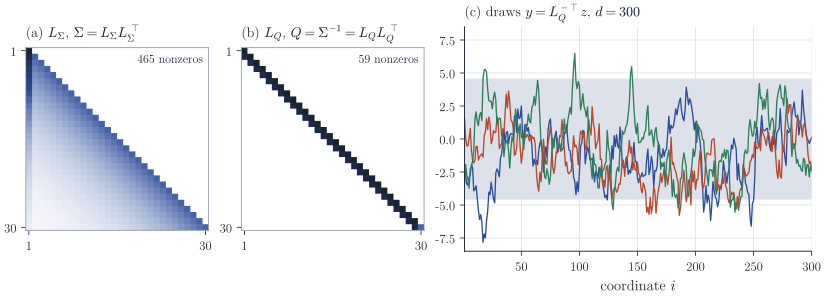
\[AA^\top = L_Q^{-\top} L_Q^{-1} = (L_Q L_Q^\top)^{-1} = Q^{-1} = \Sigma .\]In practice \(y - \mu\) is obtained by solving the upper triangular system \(L_Q^\top (y - \mu) = z\) by back-substitution. The transpose matters. The seemingly analogous choice \(A = L_Q^{-1}\) gives \(AA^\top = (L_Q^\top L_Q)^{-1}\), which differs from \(\Sigma\) unless \(L_Q^\top L_Q = L_Q L_Q^\top\), and for a triangular matrix that happens only when it is diagonal. And \(A = L_Q\) produces covariance \(Q\) itself. In the example below, \(L_Q^{-1} z\) would give the first coordinate variance \(1\) instead of \(1/(1 - \phi^2) \approx 5.3\).
If the distribution is given in the canonical form \(N(Q^{-1}b, Q^{-1})\), as in Bayesian linear regression, where \(Q = X^\top X/\sigma^2 + \Lambda_0\) and \(b = X^\top y_{\text{obs}}/\sigma^2 + \Lambda_0 m_0\) for a \(N(m_0, \Lambda_0^{-1})\) prior, the same factor also gives the mean: solve \(L_Q v = b\) and then \(L_Q^\top \mu = v\), two triangular solves.
A sparse example. A stationary autoregression \(y_1 \sim N\bigl(0, (1-\phi^2)^{-1}\bigr)\), \(y_t = \phi y_{t-1} + \varepsilon_t\) with independent \(\varepsilon_t \sim N(0, 1)\) and \(\abs{\phi} < 1\), has a dense covariance matrix \(\Sigma_{st} = \phi^{\abs{s-t}}/(1-\phi^2)\). Its joint density is proportional to
\[\exp\Bigl[-\frac12\Bigl\{(1-\phi^2)y_1^2 + \sum_{t=2}^d (y_t - \phi y_{t-1})^2\Bigr\}\Bigr],\]and expanding the square shows that \(Q\) is tridiagonal, with diagonal \((1, 1+\phi^2, \dots, 1+\phi^2, 1)\) and off-diagonal entries \(-\phi\). The Cholesky factor of a banded positive definite matrix has the same lower bandwidth, so \(L_Q\) is bidiagonal: factorization and each draw then cost \(O(d)\) operations, against \(O(d^3)\) and \(O(d^2)\) through \(\Sigma\).
When the matrix is not numerically positive definite
A covariance matrix assembled from data or from a kernel can be positive semidefinite, or positive definite in exact arithmetic but not in floating point, and the Cholesky factorization then fails. Common remedies are the following.
- Jitter: factor \(\Sigma + \varepsilon I_d\) for a small \(\varepsilon > 0\). Since the eigenvalues of \(\Sigma + \varepsilon I_d\) are \(\lambda_i + \varepsilon\), the matrix is positive definite exactly when \(\varepsilon > -\lambda_{\min}(\Sigma)\). The draws then come from \(N_d(\mu, \Sigma + \varepsilon I_d)\), so \(\varepsilon\) should be as small as the factorization allows relative to the scale of \(\Sigma\). A common strategy starts from a tiny multiple of the average diagonal entry and increases it geometrically until the factorization succeeds.
- Eigendecomposition: compute \(\Sigma = V \Lambda V^\top\), set negative eigenvalues caused by rounding to zero, and use \(A = V_r \Lambda_r^{1/2}\) built from the \(r\) positive eigenvalues. This is the appropriate route when \(\Sigma\) is genuinely singular, for example the covariance of a vector constrained to sum to zero; Proposition 1 applies with the \(d \times r\) factor and \(z \sim N_r(0, I_r)\).
- Pivoted Cholesky: a symmetric pivoting strategy that stops when the remaining diagonal is negligible, giving a low-rank factor at lower cost than an eigendecomposition.
Remarks
Standard references for the linear algebra are Golub and Van Loan, Matrix Computations, for the Cholesky factorization and its stability, and Rue and Held, Gaussian Markov Random Fields: Theory and Applications, for sampling with sparse precision matrices, including reorderings that keep the Cholesky factor sparse beyond the banded case.