Maximum a posteriori estimation
Maximum likelihood estimation uses only the data. When the data are few, the estimate can be extreme in a way that nobody would accept: a coin that lands heads in each of five tosses has maximum likelihood estimate \(\hat\theta = 1\) for its head probability, which asserts that tails is impossible. Most people would instead report a value somewhat below one, because they believe before seeing any data that coins are roughly fair. Maximum a posteriori (MAP) estimation formalizes this by maximizing the posterior density instead of the likelihood. Below I set up the estimator, work out the coin example with a Beta prior, and point out what the MAP estimate is and is not.
From likelihood to posterior
Let \(x = (x_1, \dots, x_n)\) be data with density \(p(x \mid \theta)\) for a parameter \(\theta\) in an open set \(\Theta \subseteq \R^p\). The maximum likelihood estimate maximizes \(\theta \mapsto p(x \mid \theta)\). In the Bayesian approach, \(\theta\) is given a prior density \(\pi(\theta)\) with respect to Lebesgue measure on \(\Theta\), and Bayes’ theorem gives the posterior density
\[\pi(\theta \mid x) = \frac{p(x \mid \theta)\, \pi(\theta)}{m(x)}, \qquad m(x) = \int_\Theta p(x \mid \vartheta)\, \pi(\vartheta)\, \dd\vartheta ,\]provided the marginal density \(m(x)\) is finite and positive. The MAP estimate is a maximizer of the posterior density,
\[\hat\theta_{\text{MAP}} \in \argmax_{\theta \in \Theta}\, \pi(\theta \mid x),\]assuming a maximizer exists. Since \(m(x)\) does not depend on \(\theta\) and the logarithm is increasing, it is equivalently a maximizer of \(\log p(x \mid \theta) + \log \pi(\theta)\), and the intractable integral \(m(x)\) is never needed. For i.i.d. observations with density \(f(\cdot \mid \theta)\),
\[\hat\theta_{\text{MAP}} \in \argmax_{\theta \in \Theta}\, \Bigl\{ \sum_{i=1}^n \log f(x_i \mid \theta) + \log \pi(\theta) \Bigr\}.\]Compared with maximum likelihood, the only change is the additive term \(\log \pi(\theta)\). It acts as a penalty that pulls the estimate towards regions the prior favours. Many regularized estimators are MAP estimates in disguise: in linear regression with Gaussian errors, a prior \(\beta \sim N(0, \tau^2 I)\) gives ridge regression and independent Laplace priors on the coefficients give the lasso. The sum of \(n\) log-likelihood terms grows with \(n\) while the log prior does not, so for regular models and a prior density that is positive and continuous at the truth, the influence of the prior fades as data accumulate. With few data it can matter a great deal, which is exactly the situation where it is useful.
The coin
Let \(x_1, \dots, x_n\) be independent Bernoulli(\(\theta\)) variables, with \(x_i = 1\) for heads. Write \(n_1 = \sum_i x_i\) for the number of heads and \(n_2 = n - n_1\) for the number of tails. The likelihood is
\[p(x \mid \theta) = \prod_{i=1}^n \theta^{x_i} (1-\theta)^{1 - x_i} = \theta^{n_1} (1-\theta)^{n_2}.\](If only the count \(n_1\) is recorded, its binomial probability has an extra factor \(\binom{n}{n_1}\), which does not depend on \(\theta\) and changes nothing below.) For \(0 < n_1 < n\), the log-likelihood \(n_1 \log\theta + n_2\log(1-\theta)\) is strictly concave on \((0,1)\) with derivative \(n_1/\theta - n_2/(1-\theta)\), which vanishes at \(\hat\theta_{\text{MLE}} = n_1/n\). If \(n_1 = n\) the likelihood \(\theta^n\) is increasing and the maximum over \([0,1]\) is at \(1 = n_1/n\) again. Five heads in five tosses gives \(\hat\theta_{\text{MLE}} = 1\).
The Beta prior. A prior that encodes “the coin is probably close to fair, and heads and tails are treated alike” should be symmetric about \(1/2\) with its mode there. The Beta family
\[\pi(\theta) = \frac{\theta^{\alpha-1} (1-\theta)^{\beta-1}}{B(\alpha, \beta)}, \qquad 0 < \theta < 1, \qquad B(\alpha, \beta) = \int_0^1 t^{\alpha - 1} (1-t)^{\beta - 1}\, \dd t = \frac{\Gamma(\alpha)\Gamma(\beta)}{\Gamma(\alpha+\beta)},\]with \(\alpha, \beta > 0\) and \(\Gamma(s) = \int_0^\infty t^{s-1} e^{-t}\, \dd t\), contains such priors. Its mean and variance are
\[\E\theta = \frac{\alpha}{\alpha+\beta}, \qquad \Var\theta = \frac{\alpha\beta}{(\alpha+\beta)^2(\alpha+\beta+1)},\]and when \(\alpha, \beta > 1\) the density is unimodal with mode \((\alpha-1)/(\alpha+\beta-2)\), by the same calculation as for the likelihood above. A symmetric prior \(\alpha = \beta\) has mean \(1/2\) and variance \(1/\{4(2\alpha+1)\}\), so larger \(\alpha\) expresses a firmer belief that the coin is fair. The choice \(\alpha = \beta = 1\) is the uniform distribution, and \(\alpha = \beta < 1\) gives U-shaped densities that favour strongly biased coins.
The posterior. Multiplying likelihood and prior,
\[\pi(\theta \mid x) \propto \theta^{n_1} (1-\theta)^{n_2} \cdot \theta^{\alpha-1}(1-\theta)^{\beta-1} = \theta^{n_1 + \alpha - 1} (1-\theta)^{n_2 + \beta - 1},\]which is the kernel of a Beta distribution. Since a density is determined by its kernel up to the normalizing constant,
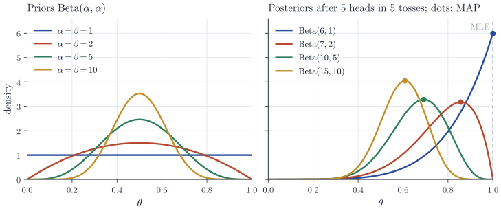
\[\theta \mid x \sim \mathrm{Beta}(n_1 + \alpha,\; n_2 + \beta).\]The prior and the posterior belong to the same family: the Beta family is conjugate to the Bernoulli likelihood. The update has a simple reading: \(\alpha\) and \(\beta\) act as pseudo-counts of heads and tails observed before the experiment, and the data add \(n_1\) and \(n_2\) to them.
Proposition 1. Let \(a = n_1 + \alpha - 1\) and \(b = n_2 + \beta - 1\), and assume \(a \ge 0\), \(b \ge 0\) and \(a + b > 0\). Then the posterior density has the unique maximizer
\[\hat\theta_{\text{MAP}} = \frac{n_1 + \alpha - 1}{n + \alpha + \beta - 2}\]over \([0, 1]\), where the density is extended to the endpoints by continuity.
Proof. Up to a positive constant the posterior density is \(g(\theta) = \theta^{a}(1-\theta)^{b}\). If \(a, b > 0\), then \(g\) vanishes at both endpoints and is positive inside, and \(\log g\) is strictly concave on \((0,1)\) with derivative
\[\frac{a}{\theta} - \frac{b}{1-\theta},\]which is zero exactly at \(\theta = a/(a+b)\). If \(b = 0 < a\), then \(g(\theta) = \theta^a\) is strictly increasing and the maximizer is \(1 = a/(a+b)\); the case \(a = 0 < b\) is symmetric.
The hypotheses matter. If \(a < 0\) or \(b < 0\), possible when \(\alpha < 1\) or \(\beta < 1\), the posterior density is unbounded near an endpoint and has no maximizer. If \(a = b = 0\), which happens for the uniform prior with no data, the posterior is uniform and every point is a maximizer.
Reading the formula
The MAP estimate is a weighted average of the sample proportion and the prior mode. When \(\alpha, \beta > 1\) and \(n \ge 1\),
\[\hat\theta_{\text{MAP}} = w\, \frac{n_1}{n} + (1-w)\, \frac{\alpha - 1}{\alpha + \beta - 2}, \qquad w = \frac{n}{n + \alpha + \beta - 2},\]as one checks by multiplying out. The prior behaves like \(\alpha + \beta - 2\) additional observations placed at the prior mode. Three special cases are worth recording.
- With no data (\(n = 0\)), the MAP estimate is the prior mode, as it should be.
- With the uniform prior \(\alpha = \beta = 1\), the posterior density is proportional to the likelihood and \(\hat\theta_{\text{MAP}} = n_1/n = \hat\theta_{\text{MLE}}\).
- With a fixed prior and \(n \to \infty\), \(w \to 1\) and \(\hat\theta_{\text{MAP}} - \hat\theta_{\text{MLE}} = O(1/n)\); the prior’s effect is of smaller order than the sampling error, which is of order \(n^{-1/2}\).
For the five heads in five tosses and a symmetric prior \(\alpha = \beta\), the MAP estimate is \((\alpha + 4)/(2\alpha + 3)\): it equals \(1\) for \(\alpha = 1\), \(6/7 \approx 0.86\) for \(\alpha = 2\), \(9/13 \approx 0.69\) for \(\alpha = 5\) and \(14/23 \approx 0.61\) for \(\alpha = 10\), and it tends to \(1/2\) as \(\alpha \to \infty\). Five observations carry little weight against a prior worth eighteen pseudo-observations.
What the MAP estimate is not
It is not invariant under reparameterization. Maximum likelihood estimates are equivariant: if \(\phi = h(\theta)\) for a bijection \(h\), the MLE of \(\phi\) is \(h(\hat\theta_{\text{MLE}})\), because the likelihood is a function and reparameterizing only relabels its argument. A posterior density, by contrast, picks up a Jacobian. For the log-odds \(\phi = \log\{\theta/(1-\theta)\}\), with inverse \(\theta = e^\phi/(1 + e^\phi)\) and \(\dd\theta/\dd\phi = \theta(1-\theta)\), the posterior density of \(\phi\) is
\[\pi_\phi(\phi \mid x) = \pi(\theta \mid x)\, \theta(1-\theta) \propto \theta^{n_1 + \alpha}(1-\theta)^{n_2 + \beta}, \qquad \theta = \frac{e^\phi}{1 + e^\phi}.\]Since \(\theta\) is an increasing function of \(\phi\), this is maximized at the \(\phi\) corresponding to \(\theta = (n_1 + \alpha)/(n + \alpha + \beta)\), which differs from the MAP estimate on the \(\theta\) scale. With the uniform prior and five heads in five tosses, the MAP estimate is \(\theta = 1\) on the probability scale and \(\phi = \log 6\), that is \(\theta = 6/7\), on the log-odds scale. The mode of a density is not a property of the distribution alone; it depends on the coordinates in which the density is written.
It is not the posterior mean. The posterior mean \((n_1 + \alpha)/(n + \alpha + \beta)\) minimizes the posterior expected squared error and is the usual Bayes estimate. It coincides with the log-odds MAP estimate above, which is special to this model, and it is never at the boundary: with the uniform prior and five heads it is \(6/7\). The MAP estimate is attractive mainly computationally, because it requires optimization rather than integration, and for that reason it is widely used in high-dimensional models where the posterior cannot be summarized in any other way. It reports a single point and no uncertainty; the full posterior, here available in closed form, gives credible intervals as well.
The Beta–Bernoulli model and conjugate analysis are treated in detail in Gelman et al., Bayesian Data Analysis, and in Hoff, A First Course in Bayesian Statistical Methods.