Bayesian inference for the normal model with conjugate priors
The normal model is the first place where Bayesian computations can be carried out completely by hand, and the three standard cases already show most of the structure of conjugate analysis. Throughout, \(x_1, \dots, x_n\) are conditionally independent given the parameters, with
\[x_i \mid \mu, \sigma^2 \sim \mathcal{N}(\mu, \sigma^2), \qquad i = 1, \dots, n,\]and we write \(D = (x_1, \dots, x_n)\), \(\bar x = n^{-1}\sum_i x_i\). The cases are: the mean \(\mu\) unknown with \(\sigma^2\) known; the variance \(\sigma^2\) unknown with \(\mu\) known; and both unknown. The first two are one-parameter problems with a one-parameter conjugate family. The third needs a joint prior, and the answer for \(\mu\) alone is no longer normal.
Conditioning in the linear Gaussian model
The one-dimensional computations below can all be done by completing the square, but it helps to see them as instances of a single fact about Gaussian vectors, the same fact that underlies the Kalman filter and Gaussian process regression. For a symmetric positive definite matrix \(\Sigma \in \R^{k \times k}\) the density of \(\mathcal{N}(m, \Sigma)\) is
\[p(z) = (2\pi)^{-k/2} (\det \Sigma)^{-1/2} \exp\Bigl(-\tfrac12 (z - m)^\top \Sigma^{-1} (z - m)\Bigr), \qquad z \in \R^k .\]Proposition 1 (Linear Gaussian model). Let \(z \sim \mathcal{N}(m, \Sigma)\) in \(\R^k\) and, conditionally on \(z\), let \(y \mid z \sim \mathcal{N}(Wz + b, \Omega)\) in \(\R^d\), where \(W \in \R^{d \times k}\), \(b \in \R^d\), and \(\Sigma\), \(\Omega\) are symmetric positive definite. Then
\[\begin{pmatrix} z \\ y \end{pmatrix} \sim \mathcal{N}\left( \begin{pmatrix} m \\ Wm + b \end{pmatrix}, \begin{pmatrix} \Sigma & \Sigma W^\top \\ W\Sigma & W\Sigma W^\top + \Omega \end{pmatrix} \right),\]and, with \(S = W\Sigma W^\top + \Omega\),
\[z \mid y \sim \mathcal{N}\Bigl( m + \Sigma W^\top S^{-1} (y - Wm - b),\; \Sigma - \Sigma W^\top S^{-1} W \Sigma \Bigr).\]Proof. The conditional law of \(y\) given \(z\) is that of \(Wz + b + \varepsilon\) with \(\varepsilon \sim \mathcal{N}(0, \Omega)\) independent of \(z\), so \((z, y)\) has the same joint law as the affine image \((z, Wz + b + \varepsilon)\) of the Gaussian vector \((z, \varepsilon)\). Affine images of Gaussian vectors are Gaussian, and the moments follow from \(\E(Wz + b + \varepsilon) = Wm + b\), \(\Cov(z, Wz + \varepsilon) = \Sigma W^\top\) and \(\Var(Wz + \varepsilon) = W\Sigma W^\top + \Omega\).
For the conditional law, put \(K = \Sigma W^\top S^{-1}\) and \(r = z - m - K(y - Wm - b)\). Then \(\Cov(r, y) = \Sigma W^\top - K S = 0\). Since \((r, y)\) is an affine image of \((z, y)\), it is jointly Gaussian, so zero covariance implies that \(r\) is independent of \(y\); its mean is zero and its covariance is \(\Sigma - \Sigma W^\top K^\top - K W \Sigma + K S K^\top = \Sigma - K S K^\top = \Sigma - \Sigma W^\top S^{-1} W \Sigma\). Writing \(z = m + K(y - Wm - b) + r\) gives the conditional distribution. Here \(S\) is invertible because \(\Omega\) is positive definite.
The second statement is Bayes’ rule for a Gaussian prior on \(z\) and a Gaussian likelihood that is linear in \(z\): the posterior is Gaussian, and its mean moves from \(m\) towards the observation by the gain \(K\).
Unknown mean, known variance
As a function of \(\mu\) the likelihood is
\[p(D \mid \mu) = (2\pi\sigma^2)^{-n/2} \exp\Bigl(-\frac{1}{2\sigma^2} \sum_{i=1}^n (x_i - \mu)^2\Bigr) \propto \exp\Bigl(-\frac{n}{2\sigma^2} (\mu - \bar x)^2\Bigr),\]where the proportionality uses \(\sum_i (x_i - \mu)^2 = \sum_i (x_i - \bar x)^2 + n(\bar x - \mu)^2\) and drops the factor that does not involve \(\mu\). The likelihood depends on the data only through \(\bar x\) and is a Gaussian kernel in \(\mu\), so a normal prior \(\mu \sim \mathcal{N}(m, \tau^2)\) is conjugate. Multiplying,
\[\begin{aligned} p(\mu \mid D) &\propto \exp\Bigl(-\frac{n}{2\sigma^2}(\mu - \bar x)^2 - \frac{1}{2\tau^2}(\mu - m)^2\Bigr) \\ &\propto \exp\Bigl(-\frac12\Bigl(\frac{n}{\sigma^2} + \frac{1}{\tau^2}\Bigr)\mu^2 + \Bigl(\frac{n \bar x}{\sigma^2} + \frac{m}{\tau^2}\Bigr)\mu\Bigr). \end{aligned}\]A density proportional to \(\exp(-\tfrac12 a \mu^2 + c\mu)\) with \(a > 0\) is the \(\mathcal{N}(c/a, 1/a)\) density, by completing the square. Hence \(\mu \mid D \sim \mathcal{N}(m_n, \tau_n^2)\) with
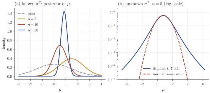
\[\frac{1}{\tau_n^2} = \frac{1}{\tau^2} + \frac{n}{\sigma^2}, \qquad m_n = \tau_n^2 \Bigl(\frac{m}{\tau^2} + \frac{n \bar x}{\sigma^2}\Bigr) = \frac{\sigma^2}{\sigma^2 + n\tau^2}\, m + \frac{n\tau^2}{\sigma^2 + n\tau^2}\, \bar x .\]Precisions add, and the posterior mean is a precision-weighted average of the prior mean and the sample mean. The same answer comes out of Proposition 1 with \(z = \mu\), \(y = \bar x\), \(W = 1\), \(b = 0\) and \(\Omega = \sigma^2/n\); using \(\bar x\) in place of the full sample is legitimate because the likelihood depends on the data only through \(\bar x\). As \(n \to \infty\) with \(\tau^2\) fixed, \(n \tau_n^2 \to \sigma^2\) and \(m_n - \bar x = \sigma^2 (m - \bar x)/(\sigma^2 + n\tau^2)\), which is of order \(1/n\) whenever \(\bar x\) stays bounded (for instance almost surely under the sampling model). The influence of the prior on the posterior mean therefore vanishes at rate \(1/n\), while the posterior standard deviation shrinks at rate \(n^{-1/2}\) (Figure 1(a)).
Unknown variance, known mean
Now \(\mu\) is known and the parameter is \(\sigma^2 > 0\). With \(S_\mu = \sum_{i=1}^n (x_i - \mu)^2\),
\[p(D \mid \sigma^2) \propto (\sigma^2)^{-n/2} \exp\Bigl(-\frac{S_\mu}{2\sigma^2}\Bigr).\]As a function of \(\sigma^2\) this is the kernel of an inverse-gamma density. The inverse-gamma distribution \(\mathrm{IG}(a, b)\) with shape \(a > 0\) and scale \(b > 0\) has density
\[p(\sigma^2) = \frac{b^a}{\Gamma(a)} (\sigma^2)^{-a-1} \exp\Bigl(-\frac{b}{\sigma^2}\Bigr), \qquad \sigma^2 > 0,\]which is the law of \(1/G\) when \(G\) has the gamma distribution with shape \(a\) and rate \(b\). With the prior \(\sigma^2 \sim \mathrm{IG}(a, b)\),
\[p(\sigma^2 \mid D) \propto (\sigma^2)^{-(a + n/2) - 1} \exp\Bigl(-\frac{b + S_\mu/2}{\sigma^2}\Bigr),\]so \(\sigma^2 \mid D \sim \mathrm{IG}(a + n/2,\, b + S_\mu/2)\). The prior acts like \(2a\) extra observations with sum of squares \(2b\). The posterior mean is \((b + S_\mu/2)/(a + n/2 - 1)\), finite when \(a + n/2 > 1\); it differs from the maximum likelihood estimator \(S_\mu/n\) by a term of order \(1/n\) whenever \(S_\mu/n\) stays bounded. Equivalently, the precision \(1/\sigma^2\) has a gamma posterior with shape \(a + n/2\) and rate \(b + S_\mu/2\).
Both parameters unknown
When \(\mu\) and \(\sigma^2\) are both unknown, a product of a normal prior for \(\mu\) and an inverse-gamma prior for \(\sigma^2\) is not conjugate: the posterior does not factor and is not of the same form. Conjugacy is restored by letting the prior spread of \(\mu\) scale with \(\sigma^2\). The normal–inverse-gamma prior \(\mathrm{NIG}(m, \kappa, a, b)\) is
\[\sigma^2 \sim \mathrm{IG}(a, b), \qquad \mu \mid \sigma^2 \sim \mathcal{N}(m, \sigma^2/\kappa),\]with \(\kappa > 0\) interpreted as a prior sample size for \(\mu\). The joint density of the parameters and the data is proportional, as a function of \((\mu, \sigma^2)\), to
\[(\sigma^2)^{-a - 1 - 1/2 - n/2} \exp\Bigl(-\frac{1}{\sigma^2}\Bigl[b + \tfrac12 \sum_{i=1}^n (x_i - \mu)^2 + \tfrac{\kappa}{2}(\mu - m)^2\Bigr]\Bigr).\]The bracket is a quadratic in \(\mu\). Put \(\kappa_n = \kappa + n\) and \(m_n = (\kappa m + n\bar x)/\kappa_n\). Expanding both sides shows
\[\sum_{i=1}^n (x_i - \mu)^2 + \kappa(\mu - m)^2 = \kappa_n (\mu - m_n)^2 + \sum_{i=1}^n (x_i - \bar x)^2 + \frac{\kappa n}{\kappa_n} (\bar x - m)^2 ;\]the coefficients of \(\mu^2\) and \(\mu\) agree by the definitions of \(\kappa_n\) and \(m_n\), and the constant terms agree because \(\kappa m^2 + n\bar x^2 - \kappa_n m_n^2 = \kappa n (\bar x - m)^2/\kappa_n\). Therefore the posterior is \(\mathrm{NIG}(m_n, \kappa_n, a_n, b_n)\) with
\[\begin{aligned} \kappa_n &= \kappa + n, & m_n &= \frac{\kappa m + n \bar x}{\kappa + n}, \\ a_n &= a + \frac n2, & b_n &= b + \frac12 \sum_{i=1}^n (x_i - \bar x)^2 + \frac{\kappa n}{2(\kappa + n)} (\bar x - m)^2 . \end{aligned}\]The scale parameter \(b_n\) collects the within-sample sum of squares and a penalty for disagreement between \(\bar x\) and the prior mean.
Proposition 2. Under the \(\mathrm{NIG}(m, \kappa, a, b)\) prior, the marginal posterior of \(\mu\) is a Student \(t\) distribution with \(2a_n\) degrees of freedom, location \(m_n\) and scale \(s_n = \sqrt{b_n/(a_n \kappa_n)}\); that is, \((\mu - m_n)/s_n \mid D \sim t_{2a_n}\).
Proof. Write \(q = b_n + \tfrac12 \kappa_n (\mu - m_n)^2\). The joint posterior density is proportional to \((\sigma^2)^{-(a_n + 1/2) - 1} e^{-q/\sigma^2}\). Integrating out \(\sigma^2\) with the inverse-gamma normalizing constant, \(\int_0^\infty v^{-c-1} e^{-q/v} \, \dd v = \Gamma(c)\, q^{-c}\) for \(c, q > 0\), gives
\[p(\mu \mid D) \propto q^{-(a_n + 1/2)} \propto \Bigl(1 + \frac{(\mu - m_n)^2}{2a_n s_n^2}\Bigr)^{-(2a_n + 1)/2},\]using \(q = b_n\bigl(1 + \kappa_n(\mu - m_n)^2/(2b_n)\bigr)\) and \(2a_n s_n^2 = 2b_n/\kappa_n\). This is the Student \(t\) kernel with \(\nu = 2a_n\) degrees of freedom, location \(m_n\) and scale \(s_n\); here \(b_n \ge b > 0\) and \(a_n > 0\), so all quantities are well defined.
Integrating over the unknown variance thickens the tails: for small \(n\) the posterior of \(\mu\) puts far more mass at several scale units from \(m_n\) than a normal density with the same scale would (Figure 1(b)). As \(n \to \infty\) the degrees of freedom grow and the normal shape returns.
A useful check is the limit \(\kappa \to 0\), \(a \to -\tfrac12\), \(b \to 0\), which corresponds to the improper prior \(p(\mu, \sigma^2) \propto 1/\sigma^2\). The posterior is proper when \(n \ge 2\) and the \(x_i\) are not all equal, and the formulas above, which remain valid for this prior, give \(m_n = \bar x\), \(2a_n = n - 1\) and \(s_n^2 = s^2/n\) with \(s^2 = (n-1)^{-1}\sum_i (x_i - \bar x)^2\), so
\[\frac{\mu - \bar x}{s/\sqrt{n}} \,\Bigm\vert\, D \sim t_{n-1} .\]The equal-tailed posterior interval for \(\mu\) coincides numerically with the classical \(t\) confidence interval, although the two statements are about different random quantities.
Remarks
Each conjugate update can be read as adding pseudo-observations: \(\kappa\) prior observations at \(m\) for the mean, and \(2a\) prior observations with sum of squares \(2b\) for the variance. This reading also shows when a conjugate prior is restrictive. Under the NIG prior, prior uncertainty about \(\mu\) is tied to the unknown \(\sigma^2\), which may not reflect real prior knowledge. With independent priors \(\mu \sim \mathcal{N}(m, \tau^2)\) and \(\sigma^2 \sim \mathrm{IG}(a, b)\) the posterior is no longer available in closed form, but both full conditionals are: \(\mu \mid \sigma^2, D\) is given by the first case and \(\sigma^2 \mid \mu, D\) by the second. That is exactly what a two-block Gibbs sampler needs.
The multivariate analogues replace the inverse-gamma distribution with the inverse-Wishart distribution and the Student \(t\) with its multivariate version. Standard references are Gelman, Carlin, Stern, Dunson, Vehtari and Rubin, Bayesian Data Analysis (Chapters 2 and 3), and Murphy, Machine Learning: A Probabilistic Perspective.