The Kalman filter as repeated Gaussian conditioning
A state-space model describes a latent process \(z_1, z_2, \dots\) that evolves over time and is seen only through noisy measurements \(y_1, y_2, \dots\). The filtering problem is to compute, at each time \(t\), the conditional distribution of the current state \(z_t\) given the measurements \(y_{1:t} = (y_1, \dots, y_t)\) received so far, and to update it cheaply when \(y_{t+1}\) arrives. In general this distribution has no finite-dimensional description. When the dynamics and the measurements are linear and all noise is Gaussian, every filtering distribution is Gaussian, and its mean and covariance satisfy a closed recursion: the Kalman filter.
The model
Let \(z_t \in \R^n\) and \(y_t \in \R^m\). The linear Gaussian state-space model is
\[z_t = F_t z_{t-1} + w_t, \qquad y_t = H_t z_t + v_t, \qquad t = 1, 2, \dots,\]with \(z_0 \sim \mathcal{N}(\mu_0, \Sigma_0)\), \(w_t \sim \mathcal{N}(0, Q_t)\) and \(v_t \sim \mathcal{N}(0, R_t)\). The matrices \(F_t \in \R^{n \times n}\) and \(H_t \in \R^{m \times n}\) are known, \(Q_t\) and \(\Sigma_0\) are symmetric positive semidefinite, and \(R_t\) is symmetric positive definite. The assumption that does the work is independence: the random vectors \(z_0, w_1, w_2, \dots, v_1, v_2, \dots\) are mutually independent.
Two consequences follow directly. Since \(z_{t-1}\) and \(y_{1:t-1}\) are functions of \((z_0, w_{1:t-1}, v_{1:t-1})\),
\[w_t \indep (z_{t-1}, y_{1:t-1}), \qquad v_t \indep (z_t, y_{1:t-1}) .\]In density notation these are the familiar statements \(p(z_t \mid z_{t-1}, y_{1:t-1}) = p(z_t \mid z_{t-1})\) and \(p(y_t \mid z_t, y_{1:t-1}) = p(y_t \mid z_t)\). Moreover, all the variables \(z_0, z_1, \dots, y_1, y_2, \dots\) are linear functions of the independent Gaussian vectors \(z_0, w_t, v_t\), so any finite collection of them is jointly Gaussian. In particular the conditional law of \(z_t\) given \(y_{1:s}\) is Gaussian, and we write
\[z_t \mid y_{1:s} \sim \mathcal{N}(\mu_{t \mid s}, \Sigma_{t \mid s}).\]The filter computes \((\mu_{t \mid t}, \Sigma_{t \mid t})\) from \((\mu_{t-1 \mid t-1}, \Sigma_{t-1 \mid t-1})\) and \(y_t\), starting from \(\mu_{0 \mid 0} = \mu_0\), \(\Sigma_{0 \mid 0} = \Sigma_0\).
Two facts about Gaussian vectors
Lemma 1 (Linear Gaussian model). If \(x \sim \mathcal{N}(\mu, \Sigma)\) in \(\R^n\) and \(y = Ax + b + \varepsilon\) with \(\varepsilon \sim \mathcal{N}(0, R)\) independent of \(x\), then
\[\begin{pmatrix} x \\ y \end{pmatrix} \sim \mathcal{N}\left( \begin{pmatrix} \mu \\ A\mu + b \end{pmatrix}, \begin{pmatrix} \Sigma & \Sigma A^\top \\ A\Sigma & A\Sigma A^\top + R \end{pmatrix} \right).\]Proof. The pair \((x, \varepsilon)\) is Gaussian with block-diagonal covariance, and \((x, y)\) is an affine function of it, hence Gaussian. The moments are \(\E y = A\mu + b\), \(\Cov(x, y) = \Cov(x, Ax) = \Sigma A^\top\) and \(\Var(y) = A\Sigma A^\top + R\), where independence kills the cross terms involving \(\varepsilon\).
Lemma 2 (Gaussian conditioning). Let
\[\begin{pmatrix} x \\ y \end{pmatrix} \sim \mathcal{N}\left( \begin{pmatrix} \mu_x \\ \mu_y \end{pmatrix}, \begin{pmatrix} \Sigma_{xx} & \Sigma_{xy} \\ \Sigma_{yx} & \Sigma_{yy} \end{pmatrix} \right)\]with \(\Sigma_{yy}\) invertible. Then \(x \sim \mathcal{N}(\mu_x, \Sigma_{xx})\), \(y \sim \mathcal{N}(\mu_y, \Sigma_{yy})\), and
\[x \mid y \sim \mathcal{N}\bigl( \mu_x + \Sigma_{xy}\Sigma_{yy}^{-1}(y - \mu_y),\; \Sigma_{xx} - \Sigma_{xy}\Sigma_{yy}^{-1}\Sigma_{yx} \bigr).\]Proof. The marginals are coordinate projections of a Gaussian vector. For the conditional law put \(r = x - \mu_x - \Sigma_{xy}\Sigma_{yy}^{-1}(y - \mu_y)\). Then \(\E r = 0\) and \(\Cov(r, y) = \Sigma_{xy} - \Sigma_{xy}\Sigma_{yy}^{-1}\Sigma_{yy} = 0\). Since \((r, y)\) is jointly Gaussian, zero covariance means \(r \indep y\), and
\[\Var(r) = \Sigma_{xx} - 2\Sigma_{xy}\Sigma_{yy}^{-1}\Sigma_{yx} + \Sigma_{xy}\Sigma_{yy}^{-1}\Sigma_{yy}\Sigma_{yy}^{-1}\Sigma_{yx} = \Sigma_{xx} - \Sigma_{xy}\Sigma_{yy}^{-1}\Sigma_{yx}.\]Given \(y\), the vector \(x = \mu_x + \Sigma_{xy}\Sigma_{yy}^{-1}(y - \mu_y) + r\) is a fixed vector plus an independent \(\mathcal{N}(0, \Var(r))\) term.
The conditional covariance does not depend on the observed value of \(y\); this is why the covariance part of the Kalman filter can be computed before any data are seen.
The recursion
Theorem 3 (Kalman filter). Under the model above, for every \(t \ge 1\):
Prediction.
\[\mu_{t \mid t-1} = F_t \mu_{t-1 \mid t-1}, \qquad \Sigma_{t \mid t-1} = F_t \Sigma_{t-1 \mid t-1} F_t^\top + Q_t .\]Update. With the innovation \(e_t\), its covariance \(S_t\) and the gain \(K_t\),
\[e_t = y_t - H_t \mu_{t \mid t-1}, \qquad S_t = H_t \Sigma_{t \mid t-1} H_t^\top + R_t, \qquad K_t = \Sigma_{t \mid t-1} H_t^\top S_t^{-1},\]the filtering moments are
\[\mu_{t \mid t} = \mu_{t \mid t-1} + K_t e_t, \qquad \Sigma_{t \mid t} = \Sigma_{t \mid t-1} - K_t S_t K_t^\top = (I - K_t H_t)\, \Sigma_{t \mid t-1} .\]Proof. Assume \(z_{t-1} \mid y_{1:t-1} \sim \mathcal{N}(\mu_{t-1 \mid t-1}, \Sigma_{t-1 \mid t-1})\); for \(t = 1\) this is the initial condition, with \(y_{1:0}\) empty.
Prediction. Because \(w_t\) is independent of \((z_{t-1}, y_{1:t-1})\), conditionally on \(y_{1:t-1}\) the vector \(w_t\) is still \(\mathcal{N}(0, Q_t)\) and independent of \(z_{t-1}\). Lemma 1, applied conditionally on \(y_{1:t-1}\) with \(x = z_{t-1}\), \(A = F_t\), \(b = 0\), \(R = Q_t\), gives the joint law of \((z_{t-1}, z_t)\) given \(y_{1:t-1}\):
\[\begin{pmatrix} z_{t-1} \\ z_t \end{pmatrix} \Bigm\vert y_{1:t-1} \sim \mathcal{N}\left( \begin{pmatrix} \mu_{t-1 \mid t-1} \\ F_t\mu_{t-1 \mid t-1} \end{pmatrix}, \begin{pmatrix} \Sigma_{t-1 \mid t-1} & \Sigma_{t-1 \mid t-1}F_t^\top \\ F_t\Sigma_{t-1 \mid t-1} & F_t\Sigma_{t-1 \mid t-1}F_t^\top + Q_t \end{pmatrix} \right).\]The marginal of the second block is the prediction step. In density form this marginalization is the Chapman–Kolmogorov equation \(p(z_t \mid y_{1:t-1}) = \int p(z_t \mid z_{t-1})\, p(z_{t-1} \mid y_{1:t-1}) \, \dd z_{t-1}\).
Update. In the same way \(v_t\) is independent of \((z_t, y_{1:t-1})\), so Lemma 1 with \(x = z_t\), \(A = H_t\), \(R = R_t\) gives
\[\begin{pmatrix} z_t \\ y_t \end{pmatrix} \Bigm\vert y_{1:t-1} \sim \mathcal{N}\left( \begin{pmatrix} \mu_{t \mid t-1} \\ H_t\mu_{t \mid t-1} \end{pmatrix}, \begin{pmatrix} \Sigma_{t \mid t-1} & \Sigma_{t \mid t-1}H_t^\top \\ H_t\Sigma_{t \mid t-1} & S_t \end{pmatrix} \right).\]The matrix \(S_t\) is positive definite because \(R_t\) is. Since \(y_{1:t} = (y_{1:t-1}, y_t)\), the conditional law of \(z_t\) given \(y_{1:t}\) is obtained by conditioning the joint law above, which is already conditional on \(y_{1:t-1}\), on the value of \(y_t\). Lemma 2 gives
\[\begin{aligned} \mu_{t \mid t} &= \mu_{t \mid t-1} + \Sigma_{t \mid t-1}H_t^\top S_t^{-1}(y_t - H_t\mu_{t \mid t-1}) = \mu_{t \mid t-1} + K_t e_t, \\ \Sigma_{t \mid t} &= \Sigma_{t \mid t-1} - \Sigma_{t \mid t-1}H_t^\top S_t^{-1} H_t \Sigma_{t \mid t-1} . \end{aligned}\]The last expression equals \(\Sigma_{t \mid t-1} - K_t H_t \Sigma_{t \mid t-1}\) by the definition of \(K_t\), and also \(\Sigma_{t \mid t-1} - K_t S_t K_t^\top\) because \(K_t S_t K_t^\top = \Sigma_{t \mid t-1}H_t^\top S_t^{-1}H_t\Sigma_{t \mid t-1}\). Induction on \(t\) completes the proof.
The update step is Bayes’ rule for a Gaussian prior \(\mathcal{N}(\mu_{t \mid t-1}, \Sigma_{t \mid t-1})\) and a linear Gaussian likelihood. The innovation \(e_t\) is the part of \(y_t\) that could not be predicted from the past, and the gain \(K_t\) decides how much of it is transferred to the state. In the scalar case with \(H_t = 1\), \(K_t = \Sigma_{t \mid t-1}/(\Sigma_{t \mid t-1} + R_t)\): the filter trusts the measurement more when the prediction is uncertain and less when the measurement noise is large.
An example
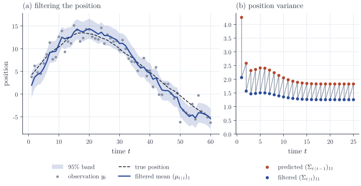
Figure 1 tracks an object on a line with the constant-velocity model: the state is \(z_t = (\text{position}, \text{velocity})\) and the measurement is the position plus noise. The acceleration is modelled as continuous-time white noise with intensity \(q\); integrating the dynamics exactly over a time step \(\Delta\) gives the transition matrix \(F\) and the noise covariance \(Q\) below. With \(\Delta = 1\),
\[F = \begin{pmatrix} 1 & \Delta \\ 0 & 1 \end{pmatrix}, \qquad Q = q\begin{pmatrix} \Delta^3/3 & \Delta^2/2 \\ \Delta^2/2 & \Delta \end{pmatrix}, \qquad H = \begin{pmatrix} 1 & 0 \end{pmatrix}, \qquad R = r,\]with \(q = 0.02\) and \(r = 4\). The velocity is never measured, yet the filter estimates it through the covariance between position and velocity that the dynamics create. Panel (b) shows the two halves of each step: prediction inflates the variance by \(F\Sigma F^\top + Q\), and the update shrinks it. The model is time-invariant, \((F, H)\) is observable and \(Q\) is positive definite, so the predicted covariance converges, from any initial \(\Sigma_0\), to the unique positive definite solution of the discrete algebraic Riccati equation
\[\Sigma = F\bigl(\Sigma - \Sigma H^\top (H\Sigma H^\top + R)^{-1} H \Sigma\bigr)F^\top + Q,\]which is the fixed-point equation obtained by composing the update and prediction steps. In the figure the covariances are within a few percent of this steady state after fifteen to twenty steps.
Remarks
The likelihood. Conditionally on \(y_{1:t-1}\), the observation \(y_t\) is \(\mathcal{N}(H_t \mu_{t \mid t-1}, S_t)\), which is the second block of the joint law in the proof. Writing \(p(y_{1:T}) = \prod_{t=1}^T p(y_t \mid y_{1:t-1})\) gives the prediction error decomposition
\[\log p(y_{1:T}) = -\frac12 \sum_{t=1}^T \Bigl( m \log(2\pi) + \log\det S_t + e_t^\top S_t^{-1} e_t \Bigr),\]which is how unknown parameters in \(F_t, H_t, Q_t, R_t\) are estimated by maximum likelihood: one filter pass evaluates the likelihood in \(O(T)\) operations.
Numerical form. In floating point arithmetic the update \(\Sigma_{t \mid t} = (I - K_t H_t)\Sigma_{t \mid t-1}\) can lose symmetry and positive semidefiniteness. The Joseph form \(\Sigma_{t \mid t} = (I - K_t H_t)\Sigma_{t \mid t-1}(I - K_t H_t)^\top + K_t R_t K_t^\top\) is algebraically equivalent when \(K_t\) is the Kalman gain, is a sum of positive semidefinite terms, and gives the correct error covariance for any gain; it is preferred in practice, as are square-root implementations that propagate a Cholesky factor of the covariance.
Beyond the linear Gaussian case. Without Gaussianity, \(\mu_{t \mid t}\) as computed by the recursion is still the best affine predictor of \(z_t\) from \(y_{1:t}\) in mean square, and \(\Sigma_{t \mid t}\) is its mean squared error matrix, provided \(z_0, w_1, w_2, \dots, v_1, v_2, \dots\) are square integrable, mutually uncorrelated, and have the stated means and covariances; the proof is the same with conditional expectations replaced by orthogonal projections in \(L^2\). In general \(\mu_{t \mid t}\) is then no longer the conditional mean. For nonlinear dynamics, the extended and unscented Kalman filters linearize or approximate the Gaussian moments, and particle filters approximate the filtering distribution by weighted samples. The backward pass that computes \(z_t \mid y_{1:T}\) for \(t < T\) is the Rauch–Tung–Striebel smoother.
The original reference is R. E. Kalman, “A new approach to linear filtering and prediction problems” (1960). Särkkä, Bayesian Filtering and Smoothing, develops the filter, the smoother and their nonlinear extensions from the same Gaussian identities, and Murphy, Probabilistic Machine Learning: Advanced Topics, places them among other inference methods for state-space models.