Autocovariance, autocorrelation and weak stationarity
A time series model specifies how observations at different times depend on each other. The coarsest useful summary of that dependence is second order: the means \(\E X_t\) and the covariances \(\Cov(X_s, X_t)\). For Gaussian processes these determine the whole distribution, and for most of classical time series analysis (ARMA modelling, spectral analysis, linear prediction) they are all that is used. What follows covers the definitions and basic properties, three standard examples, and the sampling behaviour of the sample autocorrelation function, which is the main tool for reading second-order structure from data.
Throughout, \(\{X_t : t \in \Z\}\) is a real-valued process on a probability space \((\Omega, \mathcal F, \P)\) with \(\E X_t^2 < \infty\) for every \(t\).
Autocovariance
The mean function is \(\mu_t = \E X_t\) and the autocovariance function is
\[\gamma(s, t) = \Cov(X_s, X_t) = \E\bigl[(X_s - \mu_s)(X_t - \mu_t)\bigr], \qquad s, t \in \Z,\]which is finite by the Cauchy–Schwarz inequality. Nearly every computation with autocovariances rests on bilinearity: for random variables \(U_1, \dots, U_p\) and \(V_1, \dots, V_q\) with finite second moments and real constants \(a_j, b_k\),
\[\Cov\Bigl(\sum_{j=1}^p a_j U_j, \sum_{k=1}^q b_k V_k\Bigr) = \sum_{j=1}^p \sum_{k=1}^q a_j b_k \Cov(U_j, V_k),\]which follows by expanding the product inside the expectation. In particular, for any times \(t_1, \dots, t_k\) and reals \(a_1, \dots, a_k\),
\[\sum_{i=1}^k \sum_{j=1}^k a_i a_j \gamma(t_i, t_j) = \Var\Bigl(\sum_{i=1}^k a_i X_{t_i}\Bigr) \ge 0 .\]So every autocovariance function is nonnegative definite. This is the property that characterizes autocovariance functions: any symmetric nonnegative definite function on \(\Z \times \Z\) is the autocovariance of some Gaussian process, by the Kolmogorov extension theorem.
For two processes \(X\) and \(Y\) the cross-covariance is \(\gamma_{XY}(s, t) = \Cov(X_s, Y_t)\). It need not be symmetric. If \(X\) is weakly stationary (defined below) and \(Y_t = X_{t-d}\) for a delay \(d > 0\), then \(\gamma_{XY}(t+h, t) = \gamma_X(h + d)\), which in typical cases is largest at \(h = -d\) and differs from its value at \(-h\).
Weak stationarity
Definition 1. The process \(X\) is weakly stationary (second-order stationary) if \(\mu_t = \mu\) does not depend on \(t\) and \(\gamma(t + h, t)\) does not depend on \(t\) for each \(h \in \Z\). Its autocovariance function is then the function of one variable \(\gamma(h) = \Cov(X_{t+h}, X_t)\), and if \(\gamma(0) > 0\) its autocorrelation function is
\[\rho(h) = \frac{\gamma(h)}{\gamma(0)} = \Corr(X_{t+h}, X_t), \qquad h \in \Z .\]Strict stationarity requires the joint law of \((X_{t_1 + h}, \dots, X_{t_k + h})\) to be the same for every shift \(h\). A strictly stationary process with finite second moments is weakly stationary. The converse fails in general but holds for Gaussian processes, whose finite-dimensional laws are fixed by \(\mu\) and \(\gamma\).
Proposition 2. If \(X\) is weakly stationary, then \(\gamma(0) = \Var X_t \ge 0\), \(\gamma(-h) = \gamma(h)\), \(\abs{\gamma(h)} \le \gamma(0)\), and \(\sum_{i,j=1}^k a_i a_j \gamma(i - j) \ge 0\) for all \(k\) and \(a \in \R^k\). Hence \(\rho(0) = 1\), \(\rho\) is even, and \(\abs{\rho(h)} \le 1\).
Proof. Symmetry: with \(s = t - h\), \(\gamma(-h) = \Cov(X_{t-h}, X_t) = \Cov(X_{s+h}, X_s) = \gamma(h)\), because \(\gamma(s + h, s)\) does not depend on \(s\). The bound is the Cauchy–Schwarz inequality, \(\abs{\Cov(X_{t+h}, X_t)} \le (\Var X_{t+h} \Var X_t)^{1/2} = \gamma(0)\). Nonnegative definiteness is the variance identity above with \(t_i = i\).
Weak stationarity is what makes it sensible to estimate the autocovariance from a single realization: in a series of length \(n\), the \(n - h\) pairs \((X_{t+h}, X_t)\) all have the same covariance \(\gamma(h)\), so their products can be averaged. Whether the average converges to \(\gamma(h)\) is a separate question; it requires the dependence to fade over long lags, which holds in the examples below but is not implied by weak stationarity alone (a process \(X_t = Y\) for all \(t\), with \(Y\) a single random variable, is weakly stationary).
Three examples and one non-example
Let \(\{Z_t\}\) be white noise, \(Z_t \sim \mathrm{WN}(0, \sigma^2)\): uncorrelated random variables with mean zero and variance \(\sigma^2 > 0\). Its autocovariance is \(\gamma(0) = \sigma^2\) and \(\gamma(h) = 0\) for \(h \ne 0\). White noise only requires zero correlation; an i.i.d. sequence with finite variance is white noise, but white noise need not be independent (ARCH-type processes are uncorrelated yet dependent). The distinction matters for the sample autocorrelation below.
MA(1). Let \(X_t = Z_t + \theta Z_{t-1}\). Bilinearity gives
\[\gamma(0) = \sigma^2(1 + \theta^2), \qquad \gamma(\pm 1) = \theta\sigma^2, \qquad \gamma(h) = 0 \text{ for } \abs{h} \ge 2,\]so \(\rho(1) = \theta/(1 + \theta^2)\) and the autocorrelation cuts off after lag one. Since \(1 + \theta^2 \ge 2\abs{\theta}\), \(\abs{\rho(1)} \le 1/2\): an MA(1) model cannot produce a lag-one correlation larger than one half. Also \(\theta\) and \(1/\theta\) give the same \(\rho\), so the autocorrelation alone does not identify \(\theta\); the usual convention is \(\abs{\theta} < 1\) (invertibility).
AR(1). Let \(\abs{\phi} < 1\) and consider the equation \(X_t = \phi X_{t-1} + Z_t\). Iterating it \(k\) times gives \(X_t = \sum_{j=0}^{k-1} \phi^j Z_{t-j} + \phi^k X_{t-k}\), which suggests the solution
\[X_t = \sum_{j=0}^\infty \phi^j Z_{t-j}.\]The series converges in \(L^2\) because its partial sums are Cauchy: \(\E\bigl(\sum_{j=k}^{l} \phi^j Z_{t-j}\bigr)^2 = \sigma^2 \sum_{j=k}^{l} \phi^{2j} \to 0\) as \(k, l \to \infty\). The limit satisfies the equation and is weakly stationary. It is also the only weakly stationary solution: for any such solution \(Y\), \(\E\bigl(Y_t - \sum_{j<k} \phi^j Z_{t-j}\bigr)^2 = \phi^{2k}\E Y_{t-k}^2 \to 0\). By continuity of the covariance in \(L^2\), for \(h \ge 0\),
\[\gamma(h) = \sigma^2 \sum_{j=0}^\infty \phi^{j}\phi^{j+h} = \frac{\sigma^2 \phi^h}{1 - \phi^2}, \qquad \rho(h) = \phi^{\abs{h}} .\]The autocorrelation decays geometrically and never cuts off. For \(\phi < 0\) it alternates in sign.
Random walk. With \(\phi = 1\) and \(X_0 = 0\), \(X_t = Z_1 + \dots + Z_t\) for \(t \ge 1\), and
\[\Cov(X_s, X_t) = \sigma^2 \min(s, t), \qquad s, t \ge 1 .\]The variance \(t\sigma^2\) grows linearly and the covariance depends on \(s\) and \(t\) separately, so the random walk is not weakly stationary. Its increments \(X_t - X_{t-1} = Z_t\) are; differencing is the standard way of reducing such series to stationarity.
Sample autocovariance and autocorrelation
Given observations \(X_1, \dots, X_n\) of a weakly stationary series, with \(\bar X = n^{-1}\sum_t X_t\), the sample autocovariance and autocorrelation are
\[\hat\gamma(h) = \frac1n \sum_{t=1}^{n-h} (X_{t+h} - \bar X)(X_t - \bar X), \qquad \hat\rho(h) = \frac{\hat\gamma(h)}{\hat\gamma(0)}, \qquad 0 \le h < n,\]extended by \(\hat\gamma(-h) = \hat\gamma(h)\) and \(\hat\gamma(h) = 0\) for \(\abs{h} \ge n\). The divisor is \(n\), not the number \(n - h\) of terms. This introduces a bias of order \(h/n\) but guarantees that \(\hat\gamma\) is itself nonnegative definite. Put \(Y_t = X_t - \bar X\) for \(1 \le t \le n\) and \(Y_t = 0\) otherwise. Then \(\hat\gamma(h) = n^{-1}\sum_{t \in \Z} Y_t Y_{t+h}\), so for \(a \in \R^k\)
\[\sum_{i,j=1}^k a_i a_j \hat\gamma(i - j) = \frac1n \sum_{t \in \Z} \Bigl(\sum_{i=1}^k a_i Y_{t+i}\Bigr)^2 \ge 0 ,\]where expanding the square and using \(\sum_{t} Y_{t+i} Y_{t+j} = n\hat\gamma(j - i)\) recovers the left-hand side. With divisor \(n - h\) the estimated covariance matrices can fail to be nonnegative definite, which is a problem for any procedure (Yule–Walker estimation, linear prediction) that inverts them.
The same bilinearity shows why dependence matters for the most basic estimate. For the sample mean,
\[\Var(\bar X) = \frac{1}{n^2}\sum_{s=1}^n\sum_{t=1}^n \gamma(s - t) = \frac1n \sum_{\abs{h} < n} \Bigl(1 - \frac{\abs{h}}{n}\Bigr)\gamma(h),\]since exactly \(n - \abs{h}\) pairs \((s, t)\) have \(s - t = h\). If \(\sum_h \abs{\gamma(h)} < \infty\), dominated convergence gives \(n\Var(\bar X) \to \sum_{h \in \Z}\gamma(h)\). For the AR(1) model this limit is \(\sigma^2/(1 - \phi)^2\), which is \((1 + \phi)/(1 - \phi)\) times the variance \(\gamma(0) = \sigma^2/(1 - \phi^2)\) that an independent sample of the same marginal law would give: about \(5.7\) for \(\phi = 0.7\).
Sampling behaviour of the sample autocorrelation
The sample autocorrelation is used to decide which lags carry dependence, so its sampling distribution under the absence of dependence is the natural reference.
Proposition 3. Let \(X_t = \mu + Z_t\) with \(Z_t\) i.i.d., mean zero and variance \(\sigma^2 \in (0, \infty)\). For each fixed \(H\), as \(n \to \infty\),
\[\sqrt n\,\bigl(\hat\rho(1), \dots, \hat\rho(H)\bigr) \xrightarrow{d} \mathcal{N}(0, I_H).\]Proof. The mean \(\mu\) cancels, so take \(\mu = 0\). Expanding the product in \(\hat\gamma(h)\),
\[\sqrt n\,\hat\gamma(h) = \frac{1}{\sqrt n}\sum_{t=1}^{n-h} Z_t Z_{t+h} - \bar Z\,\frac{1}{\sqrt n}\sum_{t=1}^{n-h}(Z_t + Z_{t+h}) + \frac{n-h}{\sqrt n}\,\bar Z^2 .\]By the central limit theorem \(\bar Z = O_p(n^{-1/2})\) and \(n^{-1/2}\sum_{t \le n-h}(Z_t + Z_{t+h}) = O_p(1)\), so the last two terms are \(O_p(n^{-1/2})\). The vectors \(U_t = (Z_t Z_{t+1}, \dots, Z_t Z_{t+H})\) form a strictly stationary \(H\)-dependent sequence with mean zero, and \(\E[Z_t Z_{t+h} Z_s Z_{s+k}]\) equals \(\sigma^4\) if \((s, k) = (t, h)\) and zero otherwise, because in every other case some index appears exactly once. The products have finite second moments because \(\E(Z_t Z_{t+h})^2 = \sigma^4\) by independence, so no fourth moment of \(Z_t\) is needed. The central limit theorem for strictly stationary \(m\)-dependent sequences (Brockwell and Davis, Chapter 6, prove it under finite second moments), applied to \(a^\top U_t\) for each \(a \in \R^H\) and combined with the Cramér–Wold device, gives \(n^{-1/2}\sum_{t=1}^{n} U_t \xrightarrow{d} \mathcal{N}(0, \sigma^4 I_H)\): the long-run covariance \(\sum_{l} \Cov(U_0, U_l)\) reduces to \(\Var(U_0) = \sigma^4 I_H\) by the moment computation just made. Replacing the upper limit \(n\) by \(n - h\) changes each coordinate by \(O_p(n^{-1/2})\). Finally \(\hat\gamma(0) \to \sigma^2\) almost surely by the strong law of large numbers, and Slutsky’s lemma completes the argument.
This is the source of the bands \(\pm 1.96/\sqrt n\) drawn on sample autocorrelation plots: under i.i.d. noise each \(\hat\rho(h)\) falls outside them with probability close to \(0.05\), so about one lag in twenty is expected to cross them by chance. Independence is used: for white noise that is merely uncorrelated (for example, with conditional heteroscedasticity), the variance of \(\sqrt n\,\hat\rho(h)\) can be much larger than one, and the bands understate the sampling error.
For dependent series the reference distribution changes. For a linear process \(X_t = \mu + \sum_{j \in \Z}\psi_j Z_{t-j}\) with \(\sum_j \abs{\psi_j} < \infty\) and i.i.d. \(Z_t\) having \(\E Z_t^4 < \infty\), Bartlett’s formula gives \(\sqrt n\,(\hat\rho(h) - \rho(h))_{h=1}^H \xrightarrow{d} \mathcal{N}(0, W)\) with
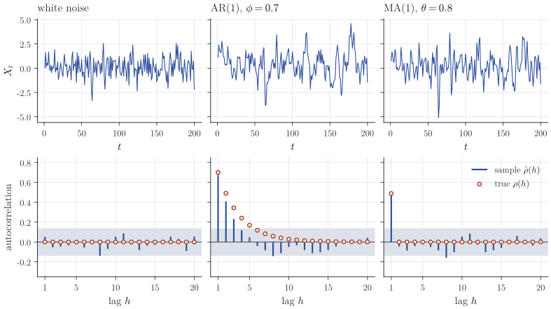
\[w_{ij} = \sum_{k=1}^\infty \bigl[\rho(k+i) + \rho(k-i) - 2\rho(i)\rho(k)\bigr]\bigl[\rho(k+j) + \rho(k-j) - 2\rho(j)\rho(k)\bigr].\]Two consequences are worth computing. For an MA(1) process and \(h \ge 2\), only \(k = h - 1, h, h + 1\) contribute and \(w_{hh} = 1 + 2\rho(1)^2\), so beyond the cut-off the sample autocorrelations are noisier than under white noise, by a factor of up to \(\sqrt{1.5}\) in standard deviation. For an AR(1) process, \(w_{11} = 1 - \phi^2\), so the lag-one sample autocorrelation is more precise than under white noise. The errors \(\hat\rho(h) - \rho(h)\) are also correlated across lags, so a sample autocorrelation function tends to wander above or below the true one over runs of consecutive lags, as in the middle panel of Figure 1.
Remarks
The two shapes in Figure 1, a cut-off after lag \(q\) and a geometric decay, are the basis of the classical identification rule: a sample autocorrelation that cuts off suggests a moving average of order \(q\), while one that decays suggests an autoregression, whose order is then read from the partial autocorrelation function. The nonnegative definiteness of \(\gamma\) is also the starting point of spectral analysis: by Herglotz’s theorem, \(\gamma\) is the sequence of Fourier coefficients of a finite measure on \((-\pi, \pi]\), the spectral measure of the process.
The material here is covered in Brockwell and Davis, Time Series: Theory and Methods (Chapters 1 and 7, the latter including Bartlett’s formula), and in Shumway and Stoffer, Time Series Analysis and Its Applications, Chapter 1.