EM for Gaussian mixture models
Gaussian mixture models are the standard model-based approach to clustering, and they are also the standard example of a likelihood that is hard to maximize directly but easy to maximize once the missing labels are imagined to be known. That is the situation the EM algorithm is designed for. Below, EM for Gaussian mixtures is worked out in full: the E-step, each part of the M-step with a proof that it is a maximizer, and the properties of the resulting iteration. The general algorithm is described in the earlier note on EM.
The model
Fix the number of components \(K\) and the dimension \(d\). A Gaussian mixture generates a point \(X \in \R^d\) in two stages. First a label is drawn,
\[Z \sim \mathrm{Categorical}(\pi_1, \dots, \pi_K), \qquad \pi_k > 0, \quad \sum_{k=1}^K \pi_k = 1,\]and then, given \(Z = k\), \(X \sim \mathcal{N}(\mu_k, \Sigma_k)\) with \(\mu_k \in \R^d\) and \(\Sigma_k\) symmetric positive definite. The parameter is \(\Theta = (\pi_1, \dots, \pi_K, \mu_1, \dots, \mu_K, \Sigma_1, \dots, \Sigma_K)\). Writing
\[\phi(x; \mu, \Sigma) = (2\pi)^{-d/2}(\det\Sigma)^{-1/2}\exp\Bigl(-\tfrac12 (x - \mu)^\top \Sigma^{-1}(x - \mu)\Bigr)\]for the normal density, the joint density of \((X, Z)\) is \(p(x, k; \Theta) = \pi_k \phi(x; \mu_k, \Sigma_k)\) and the marginal density of \(X\) is the mixture
\[p(x; \Theta) = \sum_{k=1}^K \pi_k\, \phi(x; \mu_k, \Sigma_k).\]Two features of this parametrization matter later. The labels are exchangeable: permuting the components leaves \(p(x; \Theta)\) unchanged, so \(\Theta\) is identifiable at best up to relabelling. And the components need not be well separated, in which case the mixture can be close to a model with fewer components.
Clustering from a fitted mixture
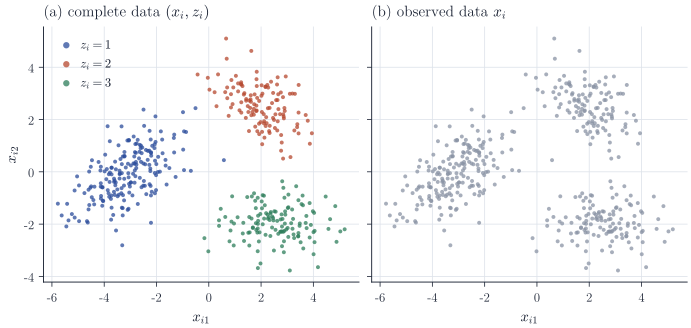
Let \(x_1, \dots, x_n \in \R^d\) be the data, modelled as i.i.d. draws from \(p(x; \Theta)\), with unobserved labels \(Z_1, \dots, Z_n\). Figure 1 shows the two views: the complete data \((x_i, z_i)\) that the model describes, and the observed data \(x_i\) that we actually have.
Given an estimate \(\hat\Theta\), Bayes’ rule gives the posterior probability that \(x_i\) came from component \(k\),
\[\P(Z_i = k \mid X_i = x_i; \hat\Theta) = \frac{\hat\pi_k\,\phi(x_i; \hat\mu_k, \hat\Sigma_k)}{\sum_{j=1}^K \hat\pi_j\,\phi(x_i; \hat\mu_j, \hat\Sigma_j)},\]and the usual hard clustering assigns \(x_i\) to the component that maximizes this probability. The posterior probabilities themselves are more informative than the hard assignment: points between two clusters receive split probabilities. Everything therefore rests on estimating \(\Theta\), which we do by maximizing the log-likelihood
\[\ell(\Theta) = \sum_{i=1}^n \log \sum_{k=1}^K \pi_k\,\phi(x_i; \mu_k, \Sigma_k).\]The logarithm of a sum does not decouple the components, and setting the gradient to zero gives no closed-form solution.
The likelihood is unbounded
Before maximizing, note that \(\ell\) has no global maximum when \(K \ge 2\). Take \(\mu_1 = x_1\) and \(\Sigma_1 = \varepsilon I\), keep the other components fixed with positive weights. The term for \(i = 1\) is at least \(\log\bigl(\pi_1 (2\pi\varepsilon)^{-d/2}\bigr)\), which tends to \(+\infty\) as \(\varepsilon \to 0\), while every other term stays bounded below by \(\log\bigl(\pi_2\,\phi(x_i; \mu_2, \Sigma_2)\bigr) > -\infty\). Hence \(\sup_\Theta \ell(\Theta) = +\infty\), approached by degenerate components that sit on single points.
The maximum likelihood estimator for Gaussian mixtures is therefore understood as a local maximizer of \(\ell\) in the interior of the parameter space. Under standard regularity conditions there is a consistent and asymptotically efficient sequence of such local maximizers, and in practice one runs EM from several starting points and keeps the best non-degenerate solution. A global maximum can be restored by constraining the covariances, for instance by requiring the eigenvalues of every \(\Sigma_j\Sigma_k^{-1}\) to be at least a fixed \(c > 0\) (Hathaway, 1985), or by placing a prior on the covariances and maximizing the posterior density instead.
The EM iteration
EM replaces the intractable \(\ell\) by a sequence of tractable problems. If the labels were observed, the complete-data log-likelihood would be
\[\log p(x_{1:n}, z_{1:n}; \Theta) = \sum_{i=1}^n \sum_{k=1}^K \mathbf 1\{z_i = k\}\bigl(\log \pi_k + \log\phi(x_i; \mu_k, \Sigma_k)\bigr),\]which separates over components. Given the current value \(\Theta_t\), EM takes the conditional expectation of this function over the unknown labels, with the labels distributed according to their posterior under \(\Theta_t\), and then maximizes in \(\Theta\).
E-step. The pairs \((X_i, Z_i)\) are independent across \(i\), so given the data the labels are independent with \(\P(Z_i = k \mid x_i; \Theta_t) = \gamma_{t,ik}\), where
\[\gamma_{t,ik} = \frac{\pi_{t,k}\,\phi(x_i; \mu_{t,k}, \Sigma_{t,k})}{\sum_{j=1}^K \pi_{t,j}\,\phi(x_i; \mu_{t,j}, \Sigma_{t,j})}\]is the responsibility of component \(k\) for point \(i\). Replacing each indicator by its conditional expectation gives
\[Q(\Theta \mid \Theta_t) = \E_{\Theta_t}\bigl[\log p(x_{1:n}, Z_{1:n}; \Theta) \mid x_{1:n}\bigr] = \sum_{i=1}^n \sum_{k=1}^K \gamma_{t,ik}\bigl(\log \pi_k + \log\phi(x_i; \mu_k, \Sigma_k)\bigr).\]M-step. Set \(\Theta_{t+1} = \argmax_\Theta Q(\Theta \mid \Theta_t)\). Write \(N_k = \sum_i \gamma_{t,ik}\) for the effective number of points in component \(k\). Then
\[Q(\Theta \mid \Theta_t) = \sum_{k=1}^K N_k \log \pi_k + \sum_{k=1}^K \sum_{i=1}^n \gamma_{t,ik}\log\phi(x_i; \mu_k, \Sigma_k),\]and the weights, and each pair \((\mu_k, \Sigma_k)\), can be optimized separately.
Proposition 1 (M-step). Suppose \(N_k > 0\) for every \(k\) and
\[S_k = \sum_{i=1}^n \gamma_{t,ik}(x_i - \bar x_k)(x_i - \bar x_k)^\top, \qquad \bar x_k = \frac{1}{N_k}\sum_{i=1}^n \gamma_{t,ik}\, x_i ,\]is positive definite for every \(k\). Then \(Q(\cdot \mid \Theta_t)\) has the unique maximizer
\[\pi_{t+1,k} = \frac{N_k}{n}, \qquad \mu_{t+1,k} = \bar x_k, \qquad \Sigma_{t+1,k} = \frac{S_k}{N_k}, \qquad k = 1, \dots, K.\]Proof. Weights. Maximize \(\sum_k N_k \log\pi_k\) subject to \(\sum_k \pi_k = 1\). The Lagrangian \(\sum_k N_k\log\pi_k + \lambda(\sum_k \pi_k - 1)\) has \(\partial/\partial\pi_k = N_k/\pi_k + \lambda\), so a stationary point has \(\pi_k = -N_k/\lambda\). Summing over \(k\) and using \(\sum_k N_k = \sum_i\sum_k\gamma_{t,ik} = n\) gives \(\lambda = -n\) and \(\pi_k = N_k/n\). The objective is strictly concave on the open simplex and the constraint is linear, so this stationary point is the unique maximizer. (Equivalently, \(\sum_k N_k\log(\pi_k n/N_k) \le n\log\sum_k \pi_k = 0\) by Jensen’s inequality.)
Means. For fixed \(\Sigma_k\), the terms involving \(\mu_k\) are \(-\tfrac12\sum_i \gamma_{t,ik}(x_i - \mu_k)^\top\Sigma_k^{-1}(x_i - \mu_k)\), a strictly concave quadratic in \(\mu_k\). Its gradient is \(\Sigma_k^{-1}\sum_i\gamma_{t,ik}(x_i - \mu_k)\), which vanishes exactly at \(\mu_k = \bar x_k\). Since this maximizer does not depend on \(\Sigma_k\), the joint maximization over \((\mu_k, \Sigma_k)\) may set \(\mu_k = \bar x_k\) first.
Covariances. With \(\mu_k = \bar x_k\) and the precision matrix \(\Lambda = \Sigma_k^{-1}\), the remaining terms are, up to a constant,
\[f(\Lambda) = \frac{N_k}{2}\log\det\Lambda - \frac12 \sum_{i=1}^n \gamma_{t,ik}(x_i - \bar x_k)^\top\Lambda(x_i - \bar x_k) = \frac{N_k}{2}\log\det\Lambda - \frac12\tr(\Lambda S_k),\]using \(v^\top\Lambda v = \tr(\Lambda vv^\top)\). Put \(C = S_k/N_k\), which is positive definite by assumption, and let \(\lambda_1, \dots, \lambda_d > 0\) be the eigenvalues of \(C^{1/2}\Lambda C^{1/2}\). Then \(\log\det\Lambda = \sum_j\log\lambda_j - \log\det C\) and \(\tr(\Lambda S_k) = N_k\tr(C^{1/2}\Lambda C^{1/2}) = N_k\sum_j\lambda_j\), so
\[f(\Lambda) = \frac{N_k}{2}\Bigl(\sum_{j=1}^d(\log\lambda_j - \lambda_j) - \log\det C\Bigr).\]Since \(\log\lambda - \lambda \le -1\) with equality only at \(\lambda = 1\), \(f\) is maximized exactly when \(C^{1/2}\Lambda C^{1/2} = I\), that is \(\Sigma_k = \Lambda^{-1} = C = S_k/N_k\).
The updates are the complete-data estimators with each point counted fractionally, with weight \(\gamma_{t,ik}\), in every component. Note that the covariance update uses the new mean \(\mu_{t+1,k}\), not \(\mu_{t,k}\).
The hypotheses of Proposition 1 hold automatically at every step if the data are not contained in an affine hyperplane of \(\R^d\) (which requires \(n \ge d + 1\)). Indeed, if \(\Theta_t\) has positive weights and positive definite covariances, every Gaussian density is positive, so every \(\gamma_{t,ik} > 0\) and \(N_k > 0\). The vectors \(x_i - \bar x_k\) then span \(\R^d\) because \(\bar x_k\) lies in the affine hull of the data, and a sum \(\sum_i\gamma_{t,ik}v_iv_i^\top\) with positive weights is positive definite when the \(v_i\) span \(\R^d\). The new \(\Theta_{t+1}\) again has positive weights and positive definite covariances, so by induction the iteration is well defined in exact arithmetic. Degeneracy can only occur in the limit, which is what the unboundedness of \(\ell\) allows.
Monotonicity
Proposition 2. Every EM step satisfies \(\ell(\Theta_{t+1}) \ge \ell(\Theta_t)\).
Proof. For any \(\Theta\) and each \(i\), \(\log p(x_i; \Theta) = \log p(x_i, k; \Theta) - \log \P(Z_i = k \mid x_i; \Theta)\) for every \(k\). Averaging over \(k\) with weights \(\gamma_{t,ik}\) and summing over \(i\),
\[\ell(\Theta) = Q(\Theta \mid \Theta_t) - \sum_{i=1}^n\sum_{k=1}^K\gamma_{t,ik}\log\P(Z_i = k \mid x_i; \Theta).\]Subtracting the same identity at \(\Theta = \Theta_t\) gives
\[\ell(\Theta) - \ell(\Theta_t) = Q(\Theta \mid \Theta_t) - Q(\Theta_t \mid \Theta_t) + \sum_{i=1}^n \KL\bigl(\P(Z_i \in \cdot \mid x_i; \Theta_t) \,\Vert\, \P(Z_i \in \cdot \mid x_i; \Theta)\bigr).\]The Kullback–Leibler divergences are nonnegative, and \(Q(\Theta_{t+1} \mid \Theta_t) \ge Q(\Theta_t \mid \Theta_t)\) by the definition of the M-step.
The identity shows more: \(Q(\cdot \mid \Theta_t) + \text{const}\) is a lower bound on \(\ell\) that touches it at \(\Theta_t\), and EM climbs \(\ell\) by maximizing that bound. Monotonicity alone does not give convergence to a maximizer. Under regularity conditions the limit points of the iteration are stationary points of \(\ell\) (Wu, 1983), usually local maxima, and which one is reached depends on the start. Near poorly separated configurations EM can also be very slow, because its rate of convergence is governed by the fraction of information that is missing.
An example
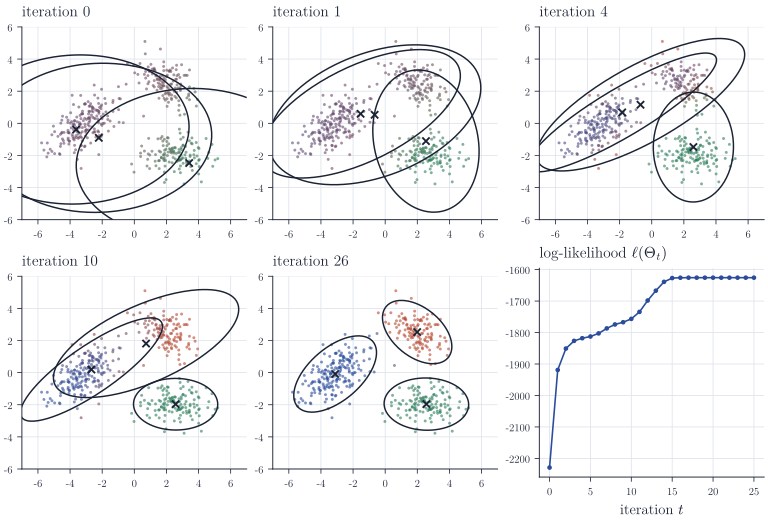
Figure 2 runs EM on the data of Figure 1 from a deliberately poor start: two of the three initial means are data points from the same cluster, and every initial covariance is the pooled sample covariance. The third component settles on the lower right cluster within a few iterations, while the two components started in the left cluster share the left and upper right clusters, both stretched along the direction joining them; during this phase the log-likelihood rises only slowly. Between iterations ten and fifteen the two stretched components separate, one of them moving to the upper right cluster, and the log-likelihood climbs to its final level. The fitted weights \((0.43, 0.28, 0.29)\) match the empirical cluster proportions, and the colour mixing in the panels shows how responsibilities are split for points between clusters.
Implementation
A direct implementation follows the formulas. Responsibilities should be computed on the log scale with the log-sum-exp function, since the densities underflow for points far from a component; the same computation yields the log-likelihood, which serves as the stopping criterion.
import numpy as np
from scipy.special import logsumexp
from scipy.stats import multivariate_normal


def em_gmm(X, weights, means, covs, max_iter=500, tol=1e-8):
    """EM for a Gaussian mixture. X has shape (n, d); the starting values
    have shapes weights (K,), means (K, d), covs (K, d, d). Returns the
    fitted parameters, the responsibilities and the log-likelihood trace."""
    n, d = X.shape
    K = len(weights)
    loglik = []
    for _ in range(max_iter):
        # E-step: log pi_k + log phi(x_i; mu_k, Sigma_k), normalized over k
        logp = np.column_stack([
            np.log(weights[k])
            + multivariate_normal.logpdf(X, means[k], covs[k])
            for k in range(K)
        ])
        ll_i = logsumexp(logp, axis=1)
        resp = np.exp(logp - ll_i[:, None])
        loglik.append(ll_i.sum())    # log-likelihood at current parameters
        if len(loglik) > 1 and loglik[-1] - loglik[-2] < tol:
            break
        # M-step (Proposition 1)
        Nk = resp.sum(axis=0)
        weights = Nk / n
        means = (resp.T @ X) / Nk[:, None]
        covs = np.empty((K, d, d))
        for k in range(K):
            D = X - means[k]               # centred at the new mean
            covs[k] = (resp[:, k, None] * D).T @ D / Nk[k]
    return weights, means, covs, resp, np.array(loglik)
The stopping rule compares successive log-likelihoods; by Proposition 2 the differences are nonnegative up to rounding. If a component collapses towards a single point during the run, its covariance becomes nearly singular and multivariate_normal.logpdf eventually raises an error. That is the unboundedness of \(\ell\) showing up in practice; the usual remedies are to restart, to bound the eigenvalues of the covariances from below, or to add a small multiple of the identity in the M-step, which corresponds to maximizing a penalized likelihood instead of \(\ell\).
Remarks
The algorithm is due in this general form to Dempster, Laird and Rubin, “Maximum likelihood from incomplete data via the EM algorithm” (1977), and its convergence theory to Wu, “On the convergence properties of the EM algorithm” (1983). Redner and Walker, “Mixture densities, maximum likelihood and the EM algorithm” (1984), treat mixtures specifically, including the local consistency of the likelihood equations, Hathaway, “A constrained formulation of maximum-likelihood estimation for normal mixture distributions” (1985), gives the constrained estimator mentioned above, and McLachlan and Peel, Finite Mixture Models, is the standard book on the subject. A stochastic variant that samples the labels in place of averaging over them is described in a later note.