From tail bounds to the Johnson–Lindenstrauss lemma: an introduction to high-dimensional statistics
Classical statistics analyses \(N\) observations \(u_1, \dots, u_N \in \R^d\) with the dimension \(d\) fixed and \(N \to \infty\). A survey that records the grade point average and nightly hours of sleep of \(N = 1000\) students has \(d = 2\), and limit theorems describe it well. The strong law of large numbers says that if \(X_1, X_2, \dots\) are i.i.d. with \(\E\abs{X_1} < \infty\), then
\[\frac1N\sum_{i=1}^N X_i \xrightarrow{\text{a.s.}} \E X_1, \qquad N \to \infty,\]and the central limit theorem says that if also \(\sigma^2 = \Var X_1 < \infty\), then \(\sqrt N\bigl(N^{-1}\sum_i X_i - \E X_1\bigr)\) converges in distribution to \(\mathcal{N}(0, \sigma^2)\).
Many modern data sets do not fit this regime. A genomic study may measure expression levels of about \(d = 20{,}000\) genes on \(N = 100\) individuals. With \(d \gg N\), a limit in which \(N \to \infty\) with \(d\) fixed says little about the data at hand. Two responses are available, and they work together. One is to prove non-asymptotic statements: inequalities valid for each finite \(N\) and \(d\), with explicit dependence on both. The other is to reduce the dimension without losing the structure of interest. Below, the basic tail inequalities behind the first approach are developed and then used to prove the Johnson–Lindenstrauss lemma, a sharp instance of the second.
Markov and Chebyshev
If \(X \ge 0\) and \(\E X\) is small, then \(X\) cannot often be large, since large values would inflate the mean.
Proposition 1 (Markov’s inequality). If \(X \ge 0\) and \(a > 0\), then \(\P(X \ge a) \le \E X / a\).
Proof. Pointwise \(X \ge X\mathbf 1\{X \ge a\} \ge a\mathbf 1\{X \ge a\}\), because \(X \ge 0\). Take expectations.
Applied to \((X - \E X)^2\), and more generally to \(\abs{X - \E X}^p\) for \(p > 0\), it gives
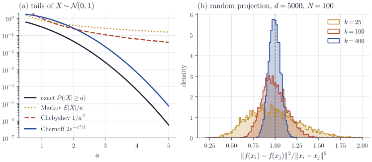
\[\P\bigl(\abs{X - \E X} \ge a\bigr) \le \frac{\Var X}{a^2}, \qquad \P\bigl(\abs{X - \E X} \ge a\bigr) \le \frac{\E\abs{X - \E X}^p}{a^p},\]the first being Chebyshev’s inequality. These bounds decay only polynomially in \(a\). For a Gaussian variable the true tail decays like \(e^{-a^2/2}\), so polynomial bounds are far too pessimistic (Figure 1(a)), and in high-dimensional problems, where thousands of events must be controlled simultaneously by a union bound, the difference is decisive.
The Chernoff bound
Proposition 2 (Chernoff bound). For any random variable \(X\) and \(a \in \R\),
\[\P(X \ge a) \le \inf_{\lambda > 0} e^{-\lambda a}\,\E e^{\lambda X},\]where terms with \(\E e^{\lambda X} = \infty\) are allowed and give the trivial bound.
Proof. For \(\lambda > 0\) the map \(x \mapsto e^{\lambda x}\) is increasing, so \(\{X \ge a\} = \{e^{\lambda X} \ge e^{\lambda a}\}\). Markov’s inequality applied to the nonnegative variable \(e^{\lambda X}\) gives \(\P(X \ge a) \le e^{-\lambda a}\E e^{\lambda X}\), and \(\lambda > 0\) is arbitrary.
No sign condition on \(X\) is needed, because the bound is applied to \(e^{\lambda X} > 0\). The moment generating function \(M(\lambda) = \E e^{\lambda X}\) carries information about all moments at once: if \(\E e^{\abs{\lambda}\abs{X}} < \infty\), then \(M(\lambda) = \sum_{k \ge 0} \lambda^k \E X^k / k!\), the interchange of sum and expectation being justified by dominated convergence with the dominating variable \(e^{\abs{\lambda}\abs{X}}\).
For \(X \sim \mathcal{N}(\mu, \sigma^2)\), \(\E e^{\lambda(X - \mu)} = e^{\sigma^2\lambda^2/2}\), so
\[\P(X - \mu \ge a) \le \inf_{\lambda > 0}\exp\Bigl(-\lambda a + \frac{\sigma^2\lambda^2}{2}\Bigr) = \exp\Bigl(-\frac{a^2}{2\sigma^2}\Bigr), \qquad a > 0,\]the infimum of the convex quadratic being attained at \(\lambda = a/\sigma^2\). Applying the same bound to \(-(X - \mu)\) and adding,
\[\P\bigl(\abs{X - \mu} \ge a\bigr) \le 2\exp\Bigl(-\frac{a^2}{2\sigma^2}\Bigr). \tag{1}\]This captures the correct exponential rate of the Gaussian tail and loses only a factor of order \(a/\sigma\) against the exact tail.
Sub-Gaussian variables and Hoeffding’s inequality
The argument for (1) used only an upper bound on the moment generating function. This motivates the following class.
Definition 3. A random variable \(X\) with mean \(\mu\) is sub-Gaussian with parameter \(\sigma > 0\) if
\[\E e^{\lambda(X - \mu)} \le e^{\sigma^2\lambda^2/2} \qquad \text{for all } \lambda \in \R .\]Every sub-Gaussian variable satisfies the tail bound (1), by the same Chernoff computation. A \(\mathcal{N}(\mu, \sigma^2)\) variable is sub-Gaussian with parameter \(\sigma\). A Rademacher variable \(\varepsilon\), equal to \(\pm 1\) with probability \(1/2\) each, is sub-Gaussian with parameter \(1\), since
\[\E e^{\lambda\varepsilon} = \cosh\lambda = \sum_{k \ge 0}\frac{\lambda^{2k}}{(2k)!} \le \sum_{k \ge 0}\frac{\lambda^{2k}}{2^k k!} = e^{\lambda^2/2},\]using \((2k)! \ge 2^k k!\). More generally, Hoeffding’s lemma states that a variable with values in \([a, b]\) is sub-Gaussian with parameter \((b - a)/2\); a proof is in the note on moment and MGF bounds.
The class is closed under independent sums. If \(X_1, \dots, X_N\) are independent and \(X_i\) is sub-Gaussian with parameter \(\sigma_i\), then by independence
\[\E\exp\Bigl(\lambda\sum_{i=1}^N (X_i - \mu_i)\Bigr) = \prod_{i=1}^N \E e^{\lambda(X_i - \mu_i)} \le \exp\Bigl(\frac{\lambda^2}{2}\sum_{i=1}^N\sigma_i^2\Bigr),\]so the centred sum is sub-Gaussian with parameter \((\sum_i\sigma_i^2)^{1/2}\). Combined with (1) and Hoeffding’s lemma this gives Hoeffding’s inequality: if the \(X_i\) are independent with \(a_i \le X_i \le b_i\), then for \(t > 0\)
\[\P\Bigl(\Bigl\lvert \sum_{i=1}^N (X_i - \E X_i)\Bigr\rvert \ge t\Bigr) \le 2\exp\Bigl(-\frac{2t^2}{\sum_{i=1}^N (b_i - a_i)^2}\Bigr).\]For the sample mean of variables in \([0, 1]\), \(\P(\abs{\bar X_N - \E\bar X_N} \ge t) \le 2e^{-2Nt^2}\): the deviation probability decays exponentially in \(N\), with no asymptotics involved.
Concentration of the chi-square distribution
The square of a Gaussian is not sub-Gaussian: if \(Z \sim \mathcal{N}(0, 1)\), then \(\E e^{\lambda Z^2} = (1 - 2\lambda)^{-1/2}\) is finite only for \(\lambda < 1/2\). Its moment generating function is, however, controlled near zero, and that is enough for the Chernoff argument as long as \(\lambda\) stays small. Variables with this property are called sub-exponential; their tails are Gaussian for moderate deviations and exponential for large ones. Bernstein’s inequality is the corresponding result for bounded variables with small variance. For the Johnson–Lindenstrauss lemma we only need the chi-square case.
Lemma 4. Let \(Z_1, \dots, Z_k\) be i.i.d. \(\mathcal{N}(0, 1)\) and \(Y = \sum_{j=1}^k Z_j^2\). For \(0 < \varepsilon \le 1\),
\[\P\bigl(\abs{Y - k} \ge \varepsilon k\bigr) \le 2\exp\Bigl(-\frac{k\varepsilon^2}{8}\Bigr).\]Proof. For \(\abs{\lambda} < 1/2\), \(\log\E e^{\lambda(Z_1^2 - 1)} = -\lambda - \tfrac12\log(1 - 2\lambda) = \sum_{j \ge 2}\frac{(2\lambda)^j}{2j}\), from the series \(-\log(1 - x) = \sum_{j \ge 1} x^j/j\). If \(\abs{\lambda} \le 1/4\), then \(\abs{2\lambda} \le 1/2\) and
\[\sum_{j \ge 2}\frac{(2\lambda)^j}{2j} \le \frac14\sum_{j \ge 2}\abs{2\lambda}^j = \frac{\lambda^2}{1 - \abs{2\lambda}} \le 2\lambda^2 .\]By independence, \(\E e^{\lambda(Y - k)} \le e^{2k\lambda^2}\) for \(\abs{\lambda} \le 1/4\). The Chernoff bound with \(0 < \lambda \le 1/4\) gives \(\P(Y - k \ge \varepsilon k) \le \exp(-\lambda\varepsilon k + 2k\lambda^2)\); the choice \(\lambda = \varepsilon/4\), admissible because \(\varepsilon \le 1\), makes the exponent \(-k\varepsilon^2/8\). The lower tail is handled in the same way with \(-\lambda\), and the two bounds add.
Since \(Y/k\) is the average of \(k\) i.i.d. variables with mean \(1\), the lemma is a quantitative law of large numbers for \(Y/k\), with deviations of relative size \(\varepsilon\) having probability at most \(2e^{-k\varepsilon^2/8}\).
The Johnson–Lindenstrauss lemma
Suppose we must store or process \(N\) points in \(\R^d\) with \(d\) very large, and the only thing that matters about them is their pairwise distances, as in nearest-neighbour search or clustering. Can they be mapped into a much lower dimension \(k\) with all distances nearly preserved? It can, and the required \(k\) depends on \(N\) and the accuracy but not on \(d\).
Theorem 5 (Johnson–Lindenstrauss). Let \(x_1, \dots, x_N \in \R^d\) with \(N \ge 2\), let \(0 < \varepsilon \le 1\) and \(0 < \delta < 1\), and let
\[k \ge \frac{8}{\varepsilon^2}\Bigl(2\log N + \log\frac1\delta\Bigr).\]Let \(A\) be a \(k \times d\) matrix with i.i.d. \(\mathcal{N}(0, 1)\) entries and \(f(x) = Ax/\sqrt k\). With probability at least \(1 - \delta\),
\[(1 - \varepsilon)\norm{x_i - x_j}^2 \le \norm{f(x_i) - f(x_j)}^2 \le (1 + \varepsilon)\norm{x_i - x_j}^2 \qquad \text{for all } i, j.\]In particular, a linear map with this property exists whenever \(k \ge 16\varepsilon^{-2}\log N\).
Proof. Fix \(u \in \R^d\) with \(u \ne 0\). The coordinates \((Au)_r = \sum_{l=1}^d A_{rl}u_l\), \(r = 1, \dots, k\), are independent, each a linear combination of independent standard normals, hence \(\mathcal{N}(0, \lVert u\rVert^2)\). Therefore \(\norm{Au}^2/\lVert u\rVert^2\) has the distribution of \(Y\) in Lemma 4, and
\[\P\Bigl(\bigl\lvert \norm{f(u)}^2 - \lVert u\rVert^2\bigr\rvert > \varepsilon\lVert u\rVert^2\Bigr) = \P\bigl(\abs{Y - k} > \varepsilon k\bigr) \le 2e^{-k\varepsilon^2/8}.\]Apply this with \(u = x_i - x_j\) for each of the at most \(N(N-1)/2\) pairs with \(x_i \ne x_j\) (pairs with \(x_i = x_j\) satisfy the conclusion trivially, since \(f\) is linear). By the union bound the probability that some pair fails is at most
\[\frac{N(N-1)}{2}\cdot 2e^{-k\varepsilon^2/8} < N^2 e^{-k\varepsilon^2/8} \le \delta,\]where the last inequality is the assumption on \(k\). For the final statement, \(k \ge 16\varepsilon^{-2}\log N\) gives \(N^2e^{-k\varepsilon^2/8} \le 1\), so the failure probability is strictly less than one and some realization of \(A\) works.
The structure of the proof is typical of high-dimensional arguments: an exponential tail bound for a single fixed object, followed by a union bound over a collection whose size enters only through a logarithm. Polynomial bounds would not survive the union bound: Chebyshev’s inequality applied to \(Y\) (with \(\Var Y = 2k\)) gives a failure probability of \(2/(k\varepsilon^2)\) per pair, which would force \(k\) to grow like \(N^2\).
Figure 1(b) shows the distortion directly. For \(N = 100\) points in \(\R^{5000}\), the ratios of squared distances after projection concentrate around \(1\) with spread of order \(\sqrt{2/k}\), the standard deviation of \(Y/k\), regardless of \(d\). The constant \(8\) in Theorem 5 is not sharp, but the order \(\varepsilon^{-2}\log N\) cannot be improved in general: Larsen and Nelson (2017) showed that there are point sets for which every linear or nonlinear map with distortion \(1 \pm \varepsilon\) needs dimension of order \(\varepsilon^{-2}\log(\varepsilon^2 N)\), provided \(\varepsilon\) is not too small relative to \(N\) and \(d\); this is of order \(\varepsilon^{-2}\log N\) unless \(\varepsilon\) is very small.
Remarks
The Gaussian matrix is convenient but not essential: matrices with i.i.d. Rademacher entries, or sparse and structured random matrices that are cheaper to apply, satisfy the same bound up to constants, because all the proof needs is a sub-exponential tail for \(\norm{Au}^2\). The lemma is due to Johnson and Lindenstrauss (1984); the short Gaussian proof above follows Dasgupta and Gupta, “An elementary proof of a theorem of Johnson and Lindenstrauss” (2003). Vershynin, High-Dimensional Probability (Chapters 2 and 5), and Wainwright, High-Dimensional Statistics: A Non-Asymptotic Viewpoint (Chapter 2), develop sub-Gaussian and sub-exponential concentration systematically and apply it far beyond random projections.