Tail bounds from moments and moment generating functions
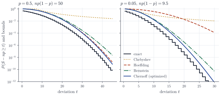
A tail bound answers the question: how likely is a random variable to be far from its mean? Such bounds are the working tools of non-asymptotic statistics. They give the accuracy of an estimator at a fixed sample size, the generalization error of a learning rule, and the sample size needed for a randomized algorithm. There are two basic routes. Moment methods apply Markov’s inequality to a power of \(\abs{X - \E X}\) and yield bounds that decay polynomially. Moment generating function (MGF) methods apply it to an exponential and yield exponential decay, provided the MGF is finite. Both routes are developed below, together with proofs of the standard inequalities for sums of independent variables and a comparison on binomial tails (Figure 1).
Moment methods
Proposition 1 (Markov’s inequality). If \(X \ge 0\) and \(t > 0\), then \(\P(X \ge t) \le \E X/t\).
Proof. Since \(X \ge 0\), \(X \ge X\mathbf 1\{X \ge t\} \ge t\,\mathbf 1\{X \ge t\}\) pointwise. Taking expectations gives \(\E X \ge t\,\P(X \ge t)\).
Markov’s inequality uses only nonnegativity and the mean, and it is sharp in that generality: for \(0 < m \le t\), the variable equal to \(t\) with probability \(m/t\) and to \(0\) otherwise has mean \(m\) and attains equality. Applying it to functions of \(X\) gives sharper bounds when more is known.
Corollary 2. Let \(\mu = \E X\). If \(\sigma^2 = \Var X < \infty\), then for \(t > 0\)
\[\P(\abs{X - \mu} \ge t) \le \frac{\sigma^2}{t^2} \qquad \text{(Chebyshev)},\]and more generally, for any \(p > 0\) with \(\E\abs{X - \mu}^p < \infty\),
\[\P(\abs{X - \mu} \ge t) \le \frac{\E\abs{X - \mu}^p}{t^p}.\]Proof. The events \(\{\abs{X - \mu} \ge t\}\) and \(\{\abs{X - \mu}^p \ge t^p\}\) coincide because \(u \mapsto u^p\) is increasing on \([0, \infty)\). Apply Markov’s inequality to \(\abs{X - \mu}^p\); the case \(p = 2\) is Chebyshev’s inequality.
The rate \(t^{-p}\) is the best that a \(p\)-th moment alone can give, and higher moments give faster polynomial decay. For variables with light tails, such as Gaussian or bounded variables, all moments are finite and the tail is in fact exponentially small, which no single moment bound can capture.
The Chernoff method
Let \(X\) have mean \(\mu\) and suppose the centred MGF is finite near zero on the right: \(\psi(\lambda) = \log\E e^{\lambda(X - \mu)} < \infty\) for \(0 \le \lambda < b\), for some \(b \in (0, \infty]\).
Proposition 3 (Chernoff bound). For every \(t \ge 0\),
\[\P(X - \mu \ge t) \le \exp\Bigl(-\sup_{0 \le \lambda < b}\bigl\{\lambda t - \psi(\lambda)\bigr\}\Bigr).\]Proof. For \(0 < \lambda < b\), the map \(u \mapsto e^{\lambda u}\) is increasing, so Markov’s inequality applied to \(e^{\lambda(X - \mu)}\) gives \(\P(X - \mu \ge t) \le e^{-\lambda t}\E e^{\lambda(X - \mu)} = e^{-(\lambda t - \psi(\lambda))}\). At \(\lambda = 0\) the bound is \(1\). Optimize over \(\lambda\).
The function \(\psi\) is convex, so \(\lambda \mapsto \lambda t - \psi(\lambda)\) is concave and the optimal \(\lambda\) is found by solving \(\psi'(\lambda) = t\) when the solution lies in \([0, b)\). The supremum is the Legendre transform of \(\psi\), the rate function of large deviations theory. Lower tails are handled by applying the bound to \(-X\).
The method is most useful for sums. If \(X_1, \dots, X_n\) are independent, then \(\E e^{\lambda\sum_i(X_i - \mu_i)} = \prod_i\E e^{\lambda(X_i - \mu_i)}\), so the exponent of the sum is the sum of the exponents. For i.i.d. \(X_i \sim \mathcal{N}(\mu, \sigma^2)\), \(\psi(\lambda) = \sigma^2\lambda^2/2\) for each term, and for the sample mean \(\bar X_n\),
\[\P(\bar X_n - \mu \ge t) = \P\Bigl(\sum_{i=1}^n(X_i - \mu) \ge nt\Bigr) \le \inf_{\lambda \ge 0}\exp\Bigl(-\lambda nt + \frac{n\sigma^2\lambda^2}{2}\Bigr) = \exp\Bigl(-\frac{nt^2}{2\sigma^2}\Bigr),\]the infimum being attained at \(\lambda = t/\sigma^2\). Since \(\bar X_n \sim \mathcal{N}(\mu, \sigma^2/n)\), the exponent is exactly that of the true tail.
Moments versus the MGF. For a nonnegative variable the optimized moment bound is never worse than the Chernoff bound. Let \(X \ge 0\) and \(\delta > 0\). By Tonelli’s theorem, for \(\lambda > 0\),
\[\E e^{\lambda X} = \sum_{k=0}^\infty\frac{\lambda^k\E X^k}{k!} = \sum_{k=0}^\infty\frac{(\lambda\delta)^k}{k!}\cdot\frac{\E X^k}{\delta^k} \ge e^{\lambda\delta}\,\inf_{k \ge 0}\frac{\E X^k}{\delta^k},\]so \(\inf_{k \ge 0}\E X^k/\delta^k \le \inf_{\lambda > 0}e^{-\lambda\delta}\E e^{\lambda X}\). The Chernoff bound is nevertheless the more useful one in practice, because MGFs factorize over independent sums while moments do not.
Hoeffding’s lemma and inequality
For bounded variables the MGF can be controlled without computing it.
Lemma 4 (Hoeffding’s lemma). If \(a \le X \le b\) almost surely and \(\E X = 0\), then for every \(\lambda \in \R\)
\[\E e^{\lambda X} \le \exp\Bigl(\frac{\lambda^2(b - a)^2}{8}\Bigr).\]Proof. Let \(F(\lambda) = \log\E e^{\lambda X}\), which is finite for all \(\lambda\) because \(X\) is bounded. Since \(\abs{X^je^{\lambda X}} \le \max(\abs a, \abs b)^j e^{\abs\lambda\max(\abs a, \abs b)}\), dominated convergence allows differentiation under the expectation, and
\[F'(\lambda) = \frac{\E[Xe^{\lambda X}]}{\E e^{\lambda X}}, \qquad F''(\lambda) = \frac{\E[X^2e^{\lambda X}]}{\E e^{\lambda X}} - \Bigl(\frac{\E[Xe^{\lambda X}]}{\E e^{\lambda X}}\Bigr)^2 .\]Thus \(F''(\lambda)\) is the variance of \(X\) under the tilted probability measure \(\P_\lambda\) with density \(e^{\lambda X}/\E e^{\lambda X}\) with respect to \(\P\). Under \(\P_\lambda\), \(X\) still takes values in \([a, b]\), and any random variable \(Y\) with values in \([a, b]\) satisfies
\[\Var(Y) \le \E\Bigl(Y - \frac{a + b}{2}\Bigr)^2 \le \Bigl(\frac{b - a}{2}\Bigr)^2,\]because the mean minimizes \(c \mapsto \E(Y - c)^2\). Hence \(F'' \le (b - a)^2/4\) everywhere. Since \(F(0) = 0\) and \(F'(0) = \E X = 0\), Taylor’s theorem with the Lagrange remainder gives \(F(\lambda) = \tfrac12 F''(\xi)\lambda^2 \le \lambda^2(b - a)^2/8\) for some \(\xi\) between \(0\) and \(\lambda\).
A sharper but less convenient bound comes from convexity. On \([a, b]\) the function \(x \mapsto e^{\lambda x}\) lies below its chord, \(e^{\lambda x} \le \frac{b - x}{b - a}e^{\lambda a} + \frac{x - a}{b - a}e^{\lambda b}\), and taking expectations with \(\E X = 0\) gives \(\E e^{\lambda X} \le (be^{\lambda a} - ae^{\lambda b})/(b - a)\). Equality holds for the two-point distribution on \(\{a, b\}\) with mean zero, so among mean-zero variables on \([a, b]\) this two-point law has the largest MGF. Lemma 4 is a clean upper bound for this extremal case.
Theorem 5 (Hoeffding’s inequality). Let \(X_1, \dots, X_n\) be independent with \(a_i \le X_i \le b_i\) almost surely, and \(S = \sum_{i=1}^n(X_i - \E X_i)\). For every \(t > 0\),
\[\P(S \ge t) \le \exp\Bigl(-\frac{2t^2}{\sum_{i=1}^n(b_i - a_i)^2}\Bigr).\]Proof. Each \(X_i - \E X_i\) has mean zero and takes values in an interval of length \(b_i - a_i\), so by independence and Lemma 4, \(\E e^{\lambda S} \le \exp(\lambda^2 D/8)\) with \(D = \sum_i(b_i - a_i)^2\). Proposition 3 gives \(\P(S \ge t) \le \exp(-\lambda t + \lambda^2D/8)\) for every \(\lambda > 0\), and the choice \(\lambda = 4t/D\) makes the exponent \(-4t^2/D + 2t^2/D = -2t^2/D\).
The same bound holds for \(\P(S \le -t)\), and for the mean of \(n\) variables in \([0, 1]\) it reads \(\P(\abs{\bar X_n - \E\bar X_n} \ge t) \le 2e^{-2nt^2}\).
Bernstein’s inequality
Hoeffding’s inequality uses only the range of each variable. When the variance is much smaller than the squared range, as for indicators of rare events, it is far from sharp. Bernstein’s inequality uses both.
Theorem 6 (Bernstein’s inequality). Let \(X_1, \dots, X_n\) be independent with \(\E X_i = 0\), \(\abs{X_i} \le M\) almost surely and \(\Var X_i = \sigma_i^2\), and let \(v = \sum_i\sigma_i^2 > 0\). For every \(t > 0\),
\[\P\Bigl(\sum_{i=1}^n X_i \ge t\Bigr) \le \exp\Bigl(-\frac{t^2}{2(v + Mt/3)}\Bigr).\]Proof. Fix \(0 < \lambda < 3/M\). For \(k \ge 2\), \(\abs{\E X_i^k} \le \E[X_i^2\abs{X_i}^{k-2}] \le \sigma_i^2M^{k-2}\), and \(k! \ge 2\cdot 3^{k-2}\) (true for \(k = 2, 3\), and the left side grows by a factor \(k \ge 3\) at each further step). Expanding the exponential, which is legitimate because \(X_i\) is bounded,
\[\begin{aligned} \E e^{\lambda X_i} &= 1 + \sum_{k \ge 2}\frac{\lambda^k\E X_i^k}{k!} \le 1 + \frac{\lambda^2\sigma_i^2}{2}\sum_{k \ge 2}\Bigl(\frac{\lambda M}{3}\Bigr)^{k-2} \\ &= 1 + \frac{\lambda^2\sigma_i^2}{2(1 - \lambda M/3)} \le \exp\Bigl(\frac{\lambda^2\sigma_i^2}{2(1 - \lambda M/3)}\Bigr). \end{aligned}\]Multiplying over \(i\) and applying Proposition 3,
\[\P\Bigl(\sum_i X_i \ge t\Bigr) \le \exp\Bigl(-\lambda t + \frac{\lambda^2v}{2(1 - \lambda M/3)}\Bigr).\]Take \(\lambda = t/(v + Mt/3)\), which satisfies \(\lambda M/3 < 1\). Then \(1 - \lambda M/3 = v/(v + Mt/3)\), the second term equals \(t^2/(2(v + Mt/3))\), the first equals \(-t^2/(v + Mt/3)\), and their sum is the stated exponent.
The bound has two regimes. For \(t \lesssim v/M\) the exponent is of order \(t^2/v\), a Gaussian tail with the true variance; for \(t \gtrsim v/M\) it is of order \(t/M\), an exponential tail set by the range. Figure 1 compares the bounds for a binomial count \(S\) with \(n = 200\), where \(X_i = B_i - p\) for i.i.d. Bernoulli(\(p\)) variables, so that \(M = \max(p, 1 - p)\) and \(v = np(1 - p)\). For \(p = 1/2\) the variance \(p(1-p) = 1/4\) is as large as the range allows, Hoeffding’s exponent \(t^2/(2v)\) is close to the optimized Chernoff exponent, and Bernstein’s bound is slightly weaker because of the extra term \(Mt/3\) in its denominator. For \(p = 0.05\) the variance per observation is more than five times smaller than this worst case, and Hoeffding’s bound, which cannot see it, is worse than Bernstein’s by almost four orders of magnitude at \(t = 20\) and by more than six at \(t = 30\).
Sub-Gaussian and sub-exponential variables
The proofs above all have the same structure: an upper bound on \(\psi(\lambda)\), followed by the Chernoff optimization. The two most common forms of the MGF bound define two classes of random variables.
Definition 7. A random variable \(X\) with mean \(\mu\) is sub-Gaussian with parameter \(\sigma > 0\) if \(\E e^{\lambda(X - \mu)} \le e^{\lambda^2\sigma^2/2}\) for all \(\lambda \in \R\). It is sub-exponential with parameters \((\nu, \alpha)\), \(\nu, \alpha > 0\), if \(\E e^{\lambda(X - \mu)} \le e^{\lambda^2\nu^2/2}\) for all \(\abs\lambda \le 1/\alpha\).
Gaussian variables are sub-Gaussian with \(\sigma\) equal to their standard deviation, and by Lemma 4 a variable with values in \([a, b]\) is sub-Gaussian with \(\sigma = (b - a)/2\). Every sub-Gaussian variable is sub-exponential, but not conversely: the MGF of \(Z^2\) for \(Z \sim \mathcal{N}(0, 1)\) is infinite for \(\lambda \ge 1/2\), yet \(Z^2\) is sub-exponential with \((\nu, \alpha) = (2, 4)\). The proof of Bernstein’s inequality shows that a variable with \(\abs{X - \mu} \le M\) and variance \(\sigma^2\) satisfies \(\psi(\lambda) \le \lambda^2\sigma^2\) for \(\abs\lambda \le 3/(2M)\), so it is sub-exponential with \((\nu, \alpha) = (\sqrt2\,\sigma, 2M/3)\), with \(\nu\) governed by the variance and not by the range.
Proposition 8. If \(X\) is sub-Gaussian with parameter \(\sigma\), then \(\P(\abs{X - \mu} \ge t) \le 2e^{-t^2/(2\sigma^2)}\) for all \(t \ge 0\). If \(X\) is sub-exponential with parameters \((\nu, \alpha)\), then
\[\P(\abs{X - \mu} \ge t) \le \begin{cases} 2e^{-t^2/(2\nu^2)}, & 0 \le t \le \nu^2/\alpha, \\ 2e^{-t/(2\alpha)}, & t > \nu^2/\alpha, \end{cases}\]that is, \(\P(\abs{X - \mu} \ge t) \le 2\exp\bigl(-\min\{t^2/(2\nu^2),\, t/(2\alpha)\}\bigr)\).
Proof. In both cases Proposition 3 gives \(\P(X - \mu \ge t) \le \exp(-\lambda t + \lambda^2\nu^2/2)\) for admissible \(\lambda \ge 0\), with \(\nu = \sigma\) in the sub-Gaussian case. The unconstrained minimizer is \(\lambda = t/\nu^2\), which gives \(e^{-t^2/(2\nu^2)}\); it is always admissible in the sub-Gaussian case, and in the sub-exponential case when \(t \le \nu^2/\alpha\). If \(t > \nu^2/\alpha\), take the boundary value \(\lambda = 1/\alpha\): since \(\nu^2/\alpha < t\), the exponent is \(-t/\alpha + \nu^2/(2\alpha^2) \le -t/\alpha + t/(2\alpha) = -t/(2\alpha)\). The lower tail follows by applying the same argument to \(-X\), and adding the two bounds gives the factor \(2\).
Both classes are closed under independent sums, with the parameters combining as in the proofs above: \(\sigma^2\) and \(\nu^2\) add, and \(\alpha\) becomes the maximum of the individual \(\alpha\)’s. Sums of sub-exponential variables therefore satisfy a Bernstein-type inequality with a Gaussian regime for small deviations and an exponential regime for large ones. This is the form in which concentration is used in high-dimensional statistics, for example in the proof of the Johnson–Lindenstrauss lemma in the note on high-dimensional tail bounds.
Remarks
Several refinements are standard. Bennett’s inequality replaces the exponent in Theorem 6 by the sharper \(\frac{v}{M^2}h(Mt/v)\) with \(h(u) = (1 + u)\log(1 + u) - u\), of which Bernstein’s bound is a simplification. For one-sided bounds with only a variance, Cantelli’s inequality \(\P(X - \mu \ge t) \le \sigma^2/(\sigma^2 + t^2)\) improves Chebyshev’s. Comprehensive treatments are Boucheron, Lugosi and Massart, Concentration Inequalities: A Nonasymptotic Theory of Independence, and Wainwright, High-Dimensional Statistics: A Non-Asymptotic Viewpoint (Chapter 2), whose sub-exponential parametrization is the one used here.