AdaBoost as stagewise minimization of the exponential loss
AdaBoost (Freund and Schapire, 1997) builds a classifier from a sequence of crude ones. Each round fits a base classifier to a reweighted version of the training data, in which the points misclassified so far carry more weight, and the final rule is a weighted vote. Stated this way the weights and vote coefficients look like design choices. Friedman, Hastie and Tibshirani (2000) observed that the algorithm is forward stagewise fitting of an additive model under the exponential loss \(e^{-yF(x)}\), and every formula in it follows from that observation. Below, the algorithm is derived from the loss; the same computation then bounds the training error and identifies what the exponential loss estimates. The last part concerns margins, which explain why the test error often keeps improving after the training error has reached zero.
Setting and the algorithm
The data are \((x_1, y_1), \dots, (x_n, y_n)\) with \(x_i\) in some space \(\mathcal X\) and labels \(y_i \in \{-1, +1\}\). Let \(\mathcal H\) be a class of base classifiers \(h : \mathcal X \to \{-1, +1\}\), closed under negation (\(h \in \mathcal H\) implies \(-h \in \mathcal H\)). Decision stumps \(h(x) = s\,\sign(x_j - t)\) with \(s \in \{-1, +1\}\) are the standard example. For probability weights \(w = (w_1, \dots, w_n)\) the weighted error of \(h\) is
\[\varepsilon(h; w) = \sum_{i=1}^n w_i\, \mathbf 1\{h(x_i) \ne y_i\} .\]AdaBoost starts from \(w^{(1)}_i = 1/n\) and, for \(m = 1, \dots, M\):
- fit \(h_m \in \mathcal H\) to the weighted data and set \(\varepsilon_m = \varepsilon(h_m; w^{(m)})\), assumed to lie in \((0, 1/2)\);
- set \(\alpha_m = \tfrac12 \log\{(1 - \varepsilon_m)/\varepsilon_m\} > 0\);
- update \(w^{(m+1)}_i = w^{(m)}_i \exp\{-\alpha_m y_i h_m(x_i)\} / Z_m\), where \(Z_m\) makes the weights sum to one.
The output is \(\sign F_M\) with \(F_M = \sum_{m=1}^M \alpha_m h_m\). Step 3 multiplies the weight of a misclassified point by \(e^{\alpha_m}\) and that of a correctly classified point by \(e^{-\alpha_m}\). The case \(\varepsilon_m = 0\) means \(h_m\) classifies the whole sample correctly and the algorithm can stop. A minimizer of the weighted error cannot have \(\varepsilon_m > 1/2\), since \(-h_m\) has weighted error \(1 - \varepsilon_m\); the case \(\varepsilon_m = 1/2\) means that no base classifier does better than random guessing on the current weights, and the algorithm stops there as well.
Unrolling step 3 from \(w^{(1)}_i = 1/n\) gives
\[\begin{equation} w^{(m+1)}_i = \frac{\exp\{-y_i F_m(x_i)\}}{n \prod_{k=1}^m Z_k}, \qquad\text{hence}\qquad \prod_{k=1}^m Z_k = \frac1n \sum_{i=1}^n \exp\{-y_i F_m(x_i)\} \label{eq:unroll} \end{equation}\]after summing over \(i\). The right-hand side is the empirical exponential risk \(L_n(F_m)\), where for any \(F : \mathcal X \to \R\)
\[L_n(F) = \frac1n \sum_{i=1}^n \exp\{-y_i F(x_i)\} .\]Derivation from the exponential loss
Forward stagewise fitting builds \(F_m = F_{m-1} + \alpha h\) by choosing the new term to reduce the risk as much as possible, without revisiting earlier terms. Under the exponential loss the previous fit enters only through weights. With \(\tilde w_i \propto \exp\{-y_i F_{m-1}(x_i)\}\) normalized to sum to one,
\[L_n(F_{m-1} + \alpha h) = L_n(F_{m-1}) \sum_{i=1}^n \tilde w_i\, e^{-\alpha y_i h(x_i)} = L_n(F_{m-1}) \Bigl\{ e^{-\alpha} + \bigl(e^{\alpha} - e^{-\alpha}\bigr)\, \varepsilon(h; \tilde w) \Bigr\},\]where the second equality uses \(y_i h(x_i) = 1\) on correctly classified points and \(-1\) on the others. On the sample, a base classifier is described by the vector \((h(x_1), \dots, h(x_n)) \in \{-1, +1\}^n\), which takes finitely many values, so the minimum of \(\varepsilon(h; \tilde w)\) over \(\mathcal H\) is attained.
Proposition 1. Suppose \(\mathcal H\) is closed under negation and \(\varepsilon_* = \min_{h \in \mathcal H} \varepsilon(h; \tilde w) \in (0, 1/2)\). Then \((\alpha, h) \mapsto L_n(F_{m-1} + \alpha h)\) over \(\alpha \ge 0\), \(h \in \mathcal H\) is minimized exactly by the pairs in which \(h\) minimizes the weighted error and \(\alpha = \tfrac12 \log\{(1 - \varepsilon_*)/\varepsilon_*\}\), and the minimum equals \(2\sqrt{\varepsilon_*(1 - \varepsilon_*)}\, L_n(F_{m-1})\). Moreover, if \(\tilde w = w^{(m)}\) then the weights \(\propto \exp\{-y_i F_m(x_i)\}\) for the next step are the AdaBoost weights \(w^{(m+1)}\).
Proof. At \(\alpha = 0\) the bracket equals \(1\). For fixed \(\alpha > 0\) the coefficient \(e^{\alpha} - e^{-\alpha}\) is positive, so the bracket is minimized by minimizing \(\varepsilon(h; \tilde w)\), giving \(g(\alpha) = (1 - \varepsilon_*) e^{-\alpha} + \varepsilon_* e^{\alpha}\). This function is strictly convex with \(g'(\alpha) = 0\) if and only if \(e^{2\alpha} = (1 - \varepsilon_*)/\varepsilon_*\), which has a positive root because \(\varepsilon_* < 1/2\). Substituting, \(g = 2\sqrt{\varepsilon_*(1-\varepsilon_*)} < 1\), so \(\alpha = 0\) is not optimal. The restriction \(\alpha \ge 0\) loses nothing, since \(\alpha h = (-\alpha)(-h)\) and \(\mathcal H\) is closed under negation. Finally, \(\exp\{-y_i F_m(x_i)\} = \exp\{-y_i F_{m-1}(x_i)\} \exp\{-\alpha_m y_i h_m(x_i)\}\), which after normalization is step 3 of the algorithm; induction from \(F_0 = 0\) gives \(\tilde w = w^{(m)}\) at every round.
So the base learner’s task of minimizing weighted error is the coordinate-selection step, and \(\alpha_m\) is an exact line search along the selected coordinate. If the base learner returns only an approximate minimizer with \(\varepsilon_m < 1/2\), the formula for \(\alpha_m\) is still the exact line search along \(h_m\). The first-order condition of that line search has a useful reading. Differentiating \(\alpha \mapsto L_n(F_{m-1} + \alpha h_m)\) at \(\alpha_m\) gives \(\sum_i w^{(m+1)}_i y_i h_m(x_i) = 0\), that is,
\[\varepsilon\bigl(h_m; w^{(m+1)}\bigr) = \tfrac12 .\]One can also check this directly: the misclassified mass after the update is \(\varepsilon_m e^{\alpha_m} / Z_m = \sqrt{\varepsilon_m(1-\varepsilon_m)} / \bigl(2\sqrt{\varepsilon_m(1-\varepsilon_m)}\bigr)\). The reweighting makes the classifier just chosen useless on the new weights, which forces the next round to find something different.
A minimal implementation, with the base learner passed in as a function returning a fitted classifier:
import numpy as np

def adaboost(X, y, fit_weighted, rounds):
    """Labels y in {-1, +1}; fit_weighted(X, y, w) returns a classifier h."""
    w = np.full(len(y), 1.0 / len(y))
    hs, alphas = [], []
    for _ in range(rounds):
        h = fit_weighted(X, y, w)
        miss = h(X) != y
        eps = w[miss].sum()
        if eps == 0 or eps >= 0.5:
            break
        alpha = 0.5 * np.log((1 - eps) / eps)
        w = w * np.exp(-alpha * y * h(X))
        w /= w.sum()
        hs.append(h); alphas.append(alpha)
    return lambda Xnew: sum(a * h(Xnew) for a, h in zip(alphas, hs))
Training error
Write \(\varepsilon_m = \tfrac12 - \gamma_m\); the edge \(\gamma_m \in (0, 1/2)\) measures how much better than random guessing \(h_m\) is on the weights it was trained on.
Theorem 2. For every \(M \ge 1\),
\[\frac1n \sum_{i=1}^n \mathbf 1\{y_i F_M(x_i) \le 0\} \;\le\; L_n(F_M) \;=\; \prod_{m=1}^M \sqrt{1 - 4\gamma_m^2} \;\le\; \exp\Bigl(-2 \sum_{m=1}^M \gamma_m^2\Bigr).\]In particular, if \(\gamma_m \ge \gamma > 0\) for all \(m\), the training error is at most \(e^{-2M\gamma^2}\), and it is zero as soon as \(M > \log n / (2\gamma^2)\).
Proof. The first inequality follows from \(\mathbf 1\{t \le 0\} \le e^{-t}\) for all real \(t\). The equality combines \(\eqref{eq:unroll}\) with \(Z_m = (1-\varepsilon_m) e^{-\alpha_m} + \varepsilon_m e^{\alpha_m} = 2\sqrt{\varepsilon_m(1-\varepsilon_m)}\) and \(4(\tfrac12 - \gamma_m)(\tfrac12 + \gamma_m) = 1 - 4\gamma_m^2\). The last inequality is \(1 - x \le e^{-x}\) applied with \(x = 4\gamma_m^2\), followed by taking square roots. For the final claim, the training error is a multiple of \(1/n\), and it is smaller than \(1/n\) once \(e^{-2M\gamma^2} < 1/n\).
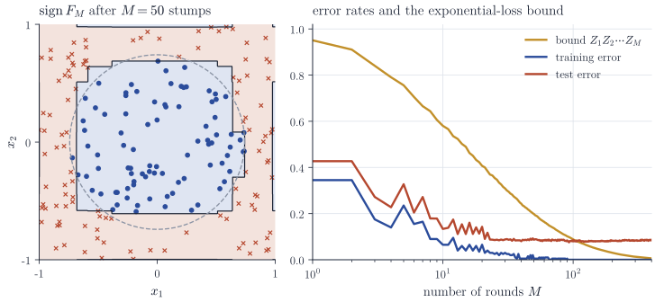
The bound requires nothing about the data or \(\mathcal H\) beyond the edges. The weak learning assumption \(\gamma_m \ge \gamma > 0\) is a condition on the pair \((\mathcal H, \text{data})\) under every reweighting that the algorithm produces, and it fails, for instance, when no combination of base classifiers can separate the sample. Figure 1 shows a run with stumps on a sample from two classes separated by a circle. The edges in that run lie between about \(0.045\) and \(0.19\), so the guarantee of Theorem 2 is conservative; the training error reaches zero after \(66\) rounds.
What the exponential loss estimates
The connection with the loss also identifies the target. Let \((X, Y)\) be a random pair with values in \(\mathcal X \times \{-1, +1\}\) and \(\eta(x) = \P(Y = 1 \mid X = x)\).
Proposition 3. Assume \(0 < \eta(X) < 1\) almost surely. Among measurable \(F : \mathcal X \to \R\), the risk \(\E \exp\{-Y F(X)\}\) is minimized by
\[F^*(x) = \frac12 \log \frac{\eta(x)}{1 - \eta(x)},\]and any other minimizer agrees with \(F^*\) for \(P_X\)-almost every \(x\). Consequently \(\sign F^*\) is a Bayes classifier.
Proof. The integrand is nonnegative, so conditioning on \(X\) is legitimate without integrability assumptions and gives \(\E \exp\{-YF(X)\} = \E\, \varphi_X(F(X))\) with \(\varphi_x(f) = \eta(x) e^{-f} + \{1 - \eta(x)\} e^{f}\). By the arithmetic–geometric mean inequality, \(\varphi_x(f) \ge 2\sqrt{\eta(x)\{1 - \eta(x)\}}\), with equality if and only if \(\eta(x) e^{-f} = \{1 - \eta(x)\} e^{f}\), that is, \(f = F^*(x)\). Hence \(\E \varphi_X(F(X)) \ge \E \varphi_X(F^*(X))\), and equality forces \(F(X) = F^*(X)\) almost surely. Finally, \(F^*(x) > 0\) exactly when \(\eta(x) > 1/2\).
Inverting, \(\eta(x) = 1/\{1 + e^{-2F^*(x)}\}\): the exponential loss estimates half the log-odds, the same target as logistic regression up to the factor \(2\). With that factor built in, the logistic loss is \(\ell(t) = \log(1 + e^{-2t})\) as a function of the margin \(t = yF\), and around \(t = 0\) both \(e^{-t}\) and \(1 - \log 2 + \ell(t)\) equal \(1 - t + t^2/2 + O(t^3)\). For \(t \to -\infty\), however, \(e^{-t}\) grows exponentially while \(\ell(t)\) grows only linearly, which makes AdaBoost sensitive to mislabelled points. When \(\eta\) takes the values \(0\) or \(1\) on a set of positive probability, as in the noiseless example of Figure 1, the population infimum is not attained. The same happens on the sample: under the weak learning assumption Theorem 2 gives \(L_n(F_M) \to 0\), hence \(y_i F_M(x_i) \to \infty\) for every \(i\), and \(F_M\) diverges on the training points.
Margins
The test error in Figure 1 stays flat for hundreds of rounds after the training error is zero, even though \(F_M\) keeps adding base classifiers. Counting base classifiers is the wrong measure of complexity here; the relevant quantity is the confidence of the vote. Let \(A_M = \sum_{m=1}^M \alpha_m\) and \(f_M = F_M / A_M\), a convex combination of base classifiers with values in \([-1, 1]\). The margin of the \(i\)th training point is \(y_i f_M(x_i)\); it is positive when the point is classified correctly and close to \(1\) when nearly all of the weighted vote is correct.
Proposition 4. For every \(\theta \in [0, 1)\),
\[\frac1n \sum_{i=1}^n \mathbf 1\{y_i f_M(x_i) \le \theta\} \;\le\; \prod_{m=1}^M 2\, \varepsilon_m^{(1-\theta)/2} (1 - \varepsilon_m)^{(1+\theta)/2} .\]If \(\varepsilon_m \le \tfrac12 - \gamma\) for all \(m\), with \(0 < \gamma < 1/2\), and \(0 \le \theta \le \gamma\), the right-hand side is at most \(\rho^M\) with \(\rho = \sqrt{(1 - 2\gamma)^{1-\theta} (1 + 2\gamma)^{1+\theta}} < 1\).
Proof. Since \(y f_M(x) \le \theta\) is equivalent to \(\theta A_M - y F_M(x) \ge 0\), we have \(\mathbf 1\{y f_M(x) \le \theta\} \le \exp\{\theta A_M - y F_M(x)\}\). Averaging and using Theorem 2,
\[\frac1n \sum_{i=1}^n \mathbf 1\{y_i f_M(x_i) \le \theta\} \le e^{\theta A_M} L_n(F_M) = \prod_{m=1}^M e^{\theta \alpha_m} Z_m ,\]and \(e^{\theta\alpha_m} Z_m = \{(1-\varepsilon_m)/\varepsilon_m\}^{\theta/2} \cdot 2\sqrt{\varepsilon_m(1-\varepsilon_m)}\) is the stated factor.
For the second claim, \(\psi(\varepsilon) = (1-\theta)\log\varepsilon + (1+\theta)\log(1-\varepsilon)\) has \(\psi'(\varepsilon) > 0\) for \(\varepsilon < (1-\theta)/2\). Because \(\theta \le \gamma < 2\gamma\), the interval \((0, \tfrac12 - \gamma]\) lies in that range, so each factor is at most its value at \(\varepsilon = \tfrac12 - \gamma\), which is \(\rho\). It remains to show \(\rho < 1\). The quantity \(\log \rho^2 = (1-\theta)\log(1-2\gamma) + (1+\theta)\log(1+2\gamma)\) is increasing in \(\theta\), so it suffices to take \(\theta = \gamma\). With \(u = 2\gamma \in (0, 1)\) and the power series of \(\log(1 - u^2)\) and \(\log\{(1+u)/(1-u)\}\),
\[\log(1 - u^2) + \frac u2 \log\frac{1+u}{1-u} = -\sum_{k\ge1} \frac{u^{2k}}{k} + \sum_{k \ge 1} \frac{u^{2k}}{2k-1} = \sum_{k \ge 2} u^{2k}\Bigl(\frac{1}{2k-1} - \frac1k\Bigr) < 0 .\]Under the weak learning assumption, therefore, the fraction of training points with margin at most \(\theta\) decays geometrically for every \(\theta \le \gamma\), not only for \(\theta = 0\). After the training error vanishes, continued boosting raises the smallest margins, as in Figure 2.
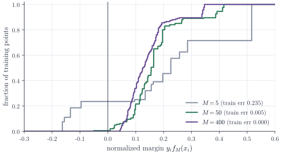
Large margins matter because of a generalization bound that does not depend on \(M\). Schapire, Freund, Bartlett and Lee (1998) proved that if \(\mathcal H\) has VC dimension \(d\) and the sample is i.i.d. from a distribution \(P\), then with probability at least \(1 - \delta\), every convex combination \(f\) of elements of \(\mathcal H\) satisfies, simultaneously for all \(\theta > 0\),
\[P\bigl(Y f(X) \le 0\bigr) \le \frac1n \sum_{i=1}^n \mathbf 1\{y_i f(x_i) \le \theta\} + \Delta_n(\theta, \delta),\]where, up to logarithmic factors in \(n\), the deviation term \(\Delta_n(\theta, \delta)\) is of order \(\sqrt{d / (n\theta^2)} + \sqrt{\log(1/\delta)/n}\). The key step approximates \(f\) by an average of a few base classifiers drawn at random from the weights \(\alpha_m / A_M\); when the margin is at least \(\theta\), roughly \(\theta^{-2}\) draws suffice to preserve the sign, so the complexity is that of short averages, whatever the number of rounds. Combined with Proposition 4, the bound says that boosting longer cannot hurt as long as it moves the margin distribution to the right.
Remarks
The margin account is not complete. Breiman (1999, Prediction games and arcing algorithms) constructed a boosting variant that provably attains larger minimum margins than AdaBoost and found that it often had higher test error, so the minimum margin alone does not determine performance; the whole margin distribution and the complexity of the base classifiers actually selected both matter. On the statistical side, Proposition 3 makes AdaBoost an estimator of half the log-odds, and with label noise it must be stopped early: Bartlett and Traskin (2007, AdaBoost is consistent) showed that stopping after a number of rounds growing suitably with \(n\) gives a Bayes-consistent procedure. Replacing the exponential loss by another convex loss in the stagewise scheme leads to gradient boosting (Friedman, 2001), where the closed-form line search of Proposition 1 is replaced by a fit to the negative gradient.
The primary sources are Freund and Schapire, A decision-theoretic generalization of on-line learning and an application to boosting (J. Comput. System Sci., 1997); Friedman, Hastie and Tibshirani, Additive logistic regression: a statistical view of boosting (Ann. Statist., 2000); and Schapire, Freund, Bartlett and Lee, Boosting the margin: a new explanation for the effectiveness of voting methods (Ann. Statist., 1998). The book by Schapire and Freund, Boosting: Foundations and Algorithms (MIT Press, 2012), treats all of the above in detail.