Uncertainty about the model itself: Bayesian model averaging for linear regression

A data analyst who selects one regression model and then reports intervals as if that model had been fixed in advance understates uncertainty: the selection step used the same data, and other models were nearly as well supported. Bayesian model averaging (BMA) treats the model as one more unknown quantity. Given a finite list of models, it assigns them prior probabilities, updates those probabilities with the data, and averages every inference over the resulting posterior. For linear regression with Zellner’s g-prior all of the required quantities are available in closed form, and a simulated example with six correlated predictors shows what averaging changes in practice.

The recipe

Let $M_1, \dots, M_K$ be candidate models. Model $M_k$ has parameter $\theta_k \in \Theta_k$, likelihood $p(D \mid \theta_k, M_k)$ and proper prior $p(\theta_k \mid M_k)$, and the models have prior probabilities $p(M_k) > 0$ summing to one. The marginal likelihood of $M_k$ is

\[p(D \mid M_k) = \int_{\Theta_k} p(D \mid \theta_k, M_k) \, p(\theta_k \mid M_k) \, \dd\theta_k ,\]

and Bayes’ theorem on the model index gives the posterior model probabilities

\[w_k := p(M_k \mid D) = \frac{p(D \mid M_k) \, p(M_k)}{\sum_{l=1}^K p(D \mid M_l) \, p(M_l)} .\]

For a quantity $\Delta$ that has the same meaning in every model, such as a future observation or a regression coefficient (set to zero in models that exclude it), the posterior is the mixture

\[p(\Delta \mid D) = \sum_{k=1}^K w_k \, p(\Delta \mid D, M_k).\]

Its mean and variance follow from the laws of total expectation and total variance:

\[\E(\Delta \mid D) = \sum_k w_k \hat\Delta_k, \qquad \Var(\Delta \mid D) = \sum_k w_k \Var(\Delta \mid D, M_k) + \sum_k w_k \bigl(\hat\Delta_k - \E(\Delta \mid D)\bigr)^2,\]

where $\hat\Delta_k = \E(\Delta \mid D, M_k)$. The second term is the part of the uncertainty that conditioning on a single selected model ignores.

The prior on $\theta_k$ within each model must be proper, or at least proper for the parameters that are not shared by all models. An improper prior is defined only up to an arbitrary constant, and that constant would enter $p(D \mid M_k)$ and hence $w_k$. Parameters common to all models, such as an intercept and the error variance below, may carry the same improper prior in every model, because the constant then cancels from the ratio.

Why average?

The mixture is the predictive distribution that the Bayesian model itself implies, and it is optimal under the logarithmic score in the following sense.

Proposition 1. Let $Y^\ast$ be a future observation and suppose the joint law of $(M, \theta_M, D, Y^\ast)$ is the one specified above, with $Y^\ast$ and $D$ conditionally independent given $(M, \theta_M)$. Let $q(\cdot \mid D)$ be any predictive density depending only on $D$, and write $p_{\mathrm{BMA}}(\cdot \mid D) = \sum_k w_k \, p(\cdot \mid D, M_k)$. If $\E\abs{\log p_{\mathrm{BMA}}(Y^\ast \mid D)} < \infty$, then

\[\E \log p_{\mathrm{BMA}}(Y^\ast \mid D) \ge \E \log q(Y^\ast \mid D),\]

with expectations taken under the joint law, the right-hand side possibly equal to $-\infty$.

Proof. Conditionally on $D$, the law of $Y^\ast$ under the joint model is

\[\sum_k p(M_k \mid D) \int p(y \mid \theta_k, M_k) \, p(\theta_k \mid D, M_k) \, \dd\theta_k = p_{\mathrm{BMA}}(y \mid D),\]

by the conditional independence assumption. Hence $\E\bigl[\log p_{\mathrm{BMA}}(Y^\ast \mid D) - \log q(Y^\ast \mid D) \mid D\bigr] = \KL\bigl(p_{\mathrm{BMA}}(\cdot \mid D) \,\Vert\, q(\cdot \mid D)\bigr) \ge 0$ by Gibbs’ inequality, and taking expectations over $D$ finishes the proof.

In particular, on average over the prior, BMA does at least as well as every rule that first selects a model from $D$ and then predicts with it. The proposition needs proper priors, so that the joint law is a probability distribution; in the regression example below the shared prior on the intercept and error variance is improper, and the proposition serves there only as a guide. The guarantee is only as good as the prior: it averages over data sets generated from the Bayesian model, not over data from a fixed true parameter. Whether BMA helps at a particular truth is an empirical question, which the simulation below examines.

Linear regression with the g-prior

Let $y \in \R^n$ and let $X$ be an $n \times p$ matrix of predictors. A model is a subset $\gamma \subseteq \{1, \dots, p\}$ of size $p_\gamma$, and $X_\gamma$ collects the corresponding columns, centred so that $\mathbf 1^\top X_\gamma = 0$. Model $M_\gamma$ states

\[y = \alpha \mathbf 1 + X_\gamma \beta_\gamma + \varepsilon, \qquad \varepsilon \sim N(0, \sigma^2 I_n),\]

with $X_\gamma^\top X_\gamma$ invertible. The prior is $p(\alpha, \sigma^2) \propto 1/\sigma^2$ in every model, shared and improper as discussed above, and Zellner’s g-prior

\[\beta_\gamma \mid \sigma^2, M_\gamma \sim N\bigl(0, \; g\sigma^2 (X_\gamma^\top X_\gamma)^{-1}\bigr), \qquad g > 0.\]

The prior covariance mimics the sampling covariance of the least-squares estimator, so $g$ measures how many “samples’ worth” of spread the prior has. We use $g = n$, the unit-information choice.

Write $\bar y$ for the mean of $y$, $y_c = y - \bar y \mathbf 1$, $\hat\beta_\gamma = (X_\gamma^\top X_\gamma)^{-1}X_\gamma^\top y_c$ and $R_\gamma^2 = y_c^\top X_\gamma\hat\beta_\gamma / y_c^\top y_c$, the coefficient of determination of the least-squares fit. Since $X_\gamma$ is centred, $\norm{y - \alpha\mathbf 1 - X_\gamma\beta_\gamma}^2 = n(\bar y - \alpha)^2 + \norm{y_c - X_\gamma\beta_\gamma}^2$, and integrating $\alpha$ over $\R$ contributes a factor $(2\pi\sigma^2/n)^{1/2}$. Next, completing the square in $\beta_\gamma$,

\[\norm{y_c - X_\gamma\beta_\gamma}^2 + \frac{\beta_\gamma^\top X_\gamma^\top X_\gamma\beta_\gamma}{g} = \frac{1+g}{g}(\beta_\gamma - m_\gamma)^\top X_\gamma^\top X_\gamma(\beta_\gamma - m_\gamma) + S_\gamma,\]

with

\[m_\gamma = \frac{g}{1+g}\hat\beta_\gamma, \qquad S_\gamma = y_c^\top y_c\Bigl(1 - \frac{g}{1+g}R_\gamma^2\Bigr).\]

The Gaussian integral over $\beta_\gamma$ cancels the prior’s normalizing constant up to a factor $(1+g)^{-p_\gamma/2}$, and the remaining integral over $\sigma^2$ is an inverse-gamma integral. Collecting terms that do not depend on $\gamma$ into a constant $C(y)$,

\[p(y \mid M_\gamma) = C(y) \, (1+g)^{-p_\gamma/2} \, S_\gamma^{-(n-1)/2}.\]

Dividing by the same expression for the intercept-only model ($p_\gamma = 0$, $S = y_c^\top y_c$) gives the Bayes factor

\[\begin{equation} \mathrm{BF}(M_\gamma : M_0) = (1+g)^{(n-1-p_\gamma)/2}\bigl(1 + g(1 - R_\gamma^2)\bigr)^{-(n-1)/2}, \label{eq:bf-g} \end{equation}\]

a function of $R^2_\gamma$, $p_\gamma$, $n$ and $g$ only. The same computation gives the within-model posteriors: $\sigma^2 \mid y, M_\gamma$ is inverse gamma with shape $(n-1)/2$ and scale $S_\gamma/2$, and $\beta_\gamma \mid y, M_\gamma$ is multivariate $t$ with $n-1$ degrees of freedom, location $m_\gamma$ and scale matrix $\frac{S_\gamma}{n-1}\cdot\frac{g}{1+g}(X_\gamma^\top X_\gamma)^{-1}$. The predictive density of a new response at a centred covariate vector $x$ is $t$ with $n-1$ degrees of freedom, location $\bar y + x_\gamma^\top m_\gamma$ and squared scale $\frac{S_\gamma}{n-1}\bigl(1 + \frac1n + \frac{g}{1+g}x_\gamma^\top(X_\gamma^\top X_\gamma)^{-1}x_\gamma\bigr)$.

Formula $\eqref{eq:bf-g}$ shows the trade-off that BMA makes. A larger $R^2_\gamma$ raises the Bayes factor, while each additional predictor costs a factor of roughly $(1+g)^{-1/2}$, which for $g = n$ is close to the $\tfrac12 \log n$ per-parameter penalty of BIC. Fernández, Ley and Steel (2001, Journal of Econometrics) compared choices of $g$, including $g = n$, and studied their consistency when the true model is among the candidates; Liang, Paulo, Molina, Clyde and Berger (2008, Journal of the American Statistical Association) pointed out that any fixed $g$ has an unpleasant limit, since $\eqref{eq:bf-g}$ stays bounded as $R^2_\gamma \to 1$, and proposed mixtures over $g$.

A simulated example

We draw $n = 60$ observations of six predictors from a centred normal distribution with unit variances, correlation 0.8 between $x_1$ and $x_2$ and correlation 0.3 between all other pairs, and set

\[y = 0.6\,x_1 + 0.4\,x_3 + 0.25\,x_6 + \varepsilon, \qquad \varepsilon \sim N(0, 1).\]

All $2^6 = 64$ subsets receive equal prior probability, and $\eqref{eq:bf-g}$ gives their posterior probabilities exactly. The most probable model, $\{x_1, x_3, x_6\}$, which is the true one, receives posterior probability only 0.28; the model $\{x_1, x_3\}$ receives 0.24, and the remaining mass is spread over models that drop $x_3$ or add one of the null predictors. A report based on the selected model would therefore condition on an event to which the posterior gives less than one chance in three.

A convenient summary of the model posterior is the posterior inclusion probability $\P(j \in \gamma \mid y) = \sum_{\gamma \ni j} w_\gamma$ (Figure 1, left). It separates the two strong effects from the three null predictors and leaves $x_6$, whose coefficient is small relative to the noise at this sample size, in between.

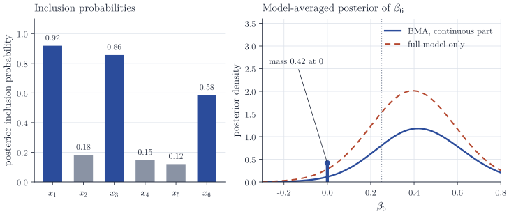
Left: posterior inclusion probabilities of six predictors. Right: model-averaged posterior of the sixth coefficient, a point mass at zero plus a continuous density, compared with the posterior under the full model — Figure 1. One simulated data set ($n = 60$, $g = n$, uniform prior over the 64 models). Left: posterior inclusion probabilities; blue bars mark predictors with nonzero true coefficients. Right: the model-averaged posterior of $\beta_6$ is a mixture of a point mass at zero, drawn as a stem whose height is its probability 0.42, and a continuous part of total mass 0.58 (solid). The dashed curve is the posterior under the full model alone; the dotted line marks the true value 0.25.

The right panel shows what averaging does to a single coefficient. Every model that excludes $x_6$ contributes a point mass at $\beta_6 = 0$, and every model that includes it contributes a $t$ density, so the averaged posterior is a spike and a smeared slab. The probability that $\beta_6 = 0$ is a statement no single-model analysis can make. The continuous part mixes posteriors from models that adjust for different sets of other predictors. Here those posteriors nearly agree, but in general the meaning of $\beta_6$ as a partial regression coefficient changes from model to model, which is a standing caveat when coefficients rather than predictions are averaged.

Does it predict better?

Proposition 1 promises better expected log predictive density under the prior. Figure 2 checks the claim at the fixed truth above. In each of 300 replications we draw a fresh training set of size 60 and a test set of size 200, and compute the mean log predictive density on the test set for the BMA mixture, for the highest-probability model, and for the full model with all six predictors.

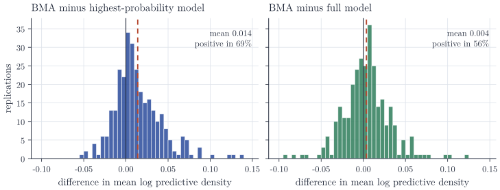
Histograms of differences in out-of-sample mean log predictive density between BMA and two single models over 300 replications — Figure 2. Differences in out-of-sample mean log predictive density over 300 replications, BMA minus the highest-probability model (left) and BMA minus the full model (right). Dashed lines mark the averages; positive values favour BMA.

The gains are real but modest: on average 0.014 nats per test observation over the highest-probability model, with BMA ahead in about 69% of replications, and 0.004 nats over the full model, ahead in 56%. This is typical. Averaging helps most when the posterior is spread over models that predict differently; when one model dominates, or when the competing models make nearly the same predictions, it reduces to model selection. With only six predictors and a strong signal, the full model is itself a reasonable predictor, and the advantage of averaging is correspondingly small.

Remarks

The model prior matters more than it appears. A uniform prior over subsets puts most of its mass on models of size near $p/2$; for larger $p$ a beta-binomial prior on the model size is a common alternative that also adjusts automatically for multiplicity. When $2^p$ is too large to enumerate, the sum over models is replaced by Markov chain Monte Carlo over $\gamma$, using the closed-form marginal likelihood $\eqref{eq:bf-g}$.

BMA is designed for the case in which one of the candidate models is regarded as true (sometimes called the $\mathcal M$-closed case). If none is, then under the usual regularity conditions the posterior model probabilities still concentrate as $n \to \infty$, on the candidate closest to the data-generating distribution in Kullback–Leibler divergence (the smallest such candidate when several nested models are equally close), and BMA reduces asymptotically to selecting that model. Minka’s note Bayesian model averaging is not model combination makes this distinction, and stacking of predictive distributions (Yao, Vehtari, Simpson and Gelman, 2018, Bayesian Analysis) is designed for the case in which a combination of models predicts better than any single one. The tutorial of Hoeting, Madigan, Raftery and Volinsky (1999, Statistical Science) remains a good general reference.