BFGS as a least-change secant update: derivation, positive definiteness and behaviour on quadratics
Newton’s method converges quadratically near a minimizer with positive definite Hessian, but every step requires second derivatives and the solution of a linear system. Gradient descent needs neither and can be extremely slow on badly scaled problems. Quasi-Newton methods sit between the two: they maintain an approximation to the inverse Hessian built only from observed changes in the gradient, and they typically converge superlinearly at the cost of first-order information. BFGS, named after Broyden, Fletcher, Goldfarb and Shanno, who proposed it independently in 1970, is the most widely used of them. Its update can be derived from a single least-change principle, and two properties follow with short proofs: it preserves positive definiteness, and on a quadratic it rebuilds the inverse Hessian in finitely many steps.
Throughout, \(f : \R^n \to \R\) is twice continuously differentiable, \(g_k = \nabla f(x_k)\), and iterates take the form
\[x_{k+1} = x_k + \alpha_k p_k, \qquad p_k = -H_k g_k ,\]with \(H_k\) symmetric positive definite and a step length \(\alpha_k > 0\) from a line search. Positive definiteness of \(H_k\) makes \(p_k\) a descent direction whenever \(g_k \neq 0\), since \(g_k^\top p_k = -g_k^\top H_k g_k < 0\).
The secant equation and the curvature condition
Write \(s_k = x_{k+1} - x_k\) and \(y_k = g_{k+1} - g_k\). By the fundamental theorem of calculus applied to \(t \mapsto \nabla f(x_k + ts_k)\),
\[y_k = \bar G_k s_k, \qquad \bar G_k = \int_0^1 \nabla^2 f(x_k + t s_k)\, \dd t ,\]so the pair \((s_k, y_k)\) reveals how the average Hessian along the step acts on \(s_k\). A quasi-Newton method asks the next approximation \(B_{k+1} \approx \nabla^2 f\) to reproduce this, \(B_{k+1}s_k = y_k\), or in terms of the inverse \(H_{k+1} = B_{k+1}^{-1}\),
\[H_{k+1}\, y_k = s_k \qquad\text{(secant equation)}.\]If \(H_{k+1}\) is positive definite, then \(s_k^\top y_k = y_k^\top H_{k+1} y_k > 0\) for \(y_k \neq 0\). The curvature condition \(s_k^\top y_k > 0\) is therefore necessary for a positive definite solution. It holds automatically when \(f\) is strictly convex, but not in general; the line search has to enforce it.
Lemma 1. If \(g_k^\top p_k < 0\) and \(\alpha_k\) satisfies the curvature part of the Wolfe conditions, \(\nabla f(x_k + \alpha_k p_k)^\top p_k \ge c_2\, g_k^\top p_k\) for some \(c_2 \in (0, 1)\), then \(s_k^\top y_k > 0\).
Proof. \(s_k^\top y_k = \alpha_k (g_{k+1} - g_k)^\top p_k \ge \alpha_k (c_2 - 1)\, g_k^\top p_k > 0\), because \(\alpha_k > 0\), \(c_2 < 1\) and \(g_k^\top p_k < 0\).
The Wolfe conditions combine this with a sufficient-decrease condition \(f(x_k + \alpha p_k) \le f(x_k) + c_1\alpha g_k^\top p_k\), \(0 < c_1 < c_2 < 1\). If \(f\) is bounded below along the ray, step lengths satisfying both exist and can be found by a simple bracketing search (Nocedal and Wright, Numerical Optimization, Chapter 3).
The update
The secant equation imposes \(n\) conditions on the \(n(n+1)/2\) free entries of a symmetric matrix, so for \(n > 1\) it does not determine \(H_{k+1}\). BFGS takes the solution closest to \(H_k\) in a particular norm. Drop the index \(k\) and write \(H\), \(s\), \(y\) for the current quantities, with \(s^\top y > 0\) and \(\rho = 1/(s^\top y)\). The norm is built from a symmetric positive definite \(W\) with \(Ws = y\); such a matrix exists exactly when \(s^\top y > 0\), for instance \(W = yy^\top/(s^\top y) + I - ss^\top/(s^\top s)\), which maps \(s\) to \(y\) and satisfies \(z^\top W z = (y^\top z)^2/(s^\top y) + \norm{z}^2 - (s^\top z)^2/\norm{s}^2 > 0\) for \(z \neq 0\) by the Cauchy–Schwarz inequality, equality in which forces \(z \parallel s\) and then \(y^\top z \neq 0\).
Theorem 2 (least-change characterization). Let \(W\) be any symmetric positive definite matrix with \(Ws = y\), and \(\lVert M\rVert_W = \lVert W^{1/2} M W^{1/2}\rVert_F\). Among symmetric matrices \(H_+\) satisfying \(H_+ y = s\), the unique minimizer of \(\lVert H_+ - H\rVert_W\), for every such \(W\), is
\[H_+ = (I - \rho\, s y^\top)\, H\, (I - \rho\, y s^\top) + \rho\, s s^\top .\]Proof. Change variables to \(\hat H = W^{1/2}H_+W^{1/2}\) and \(\hat H_0 = W^{1/2}HW^{1/2}\), and put \(u = W^{1/2}s\). Because \(Ws = y\), we have \(W^{-1/2}y = W^{1/2}s = u\), so the constraint \(H_+y = s\) becomes \(\hat H u = u\), and the objective becomes \(\lVert \hat H - \hat H_0\rVert_F\). Let \(P = uu^\top/(u^\top u)\) and \(P_\perp = I - P\). A symmetric \(\hat H\) with \(\hat Hu = u\) also satisfies \(u^\top\hat H = u^\top\), hence \(\hat H P = P\hat H = P\) and
\[\hat H = P + P_\perp \hat H P_\perp .\]The Frobenius norm splits over the four blocks \(P(\cdot)P\), \(P(\cdot)P_\perp\), \(P_\perp(\cdot)P\), \(P_\perp(\cdot)P_\perp\), which are orthogonal in the trace inner product. Only the last block of \(\hat H - \hat H_0\) depends on the free part \(P_\perp\hat HP_\perp\), so the unique minimizer is \(\hat H = P + P_\perp \hat H_0 P_\perp\). Transforming back, \(u^\top u = s^\top W s = s^\top y\) gives \(W^{-1/2}PW^{-1/2} = \rho\, ss^\top\), and \(W^{-1/2}P_\perp W^{1/2} = I - \rho\, W^{-1/2}u\,u^\top W^{1/2} = I - \rho\, s y^\top\), since \(W^{-1/2}u = s\) and \(u^\top W^{1/2} = s^\top W = y^\top\). Therefore
\[H_+ = W^{-1/2}\bigl(P + P_\perp \hat H_0 P_\perp\bigr)W^{-1/2} = \rho\, ss^\top + (I - \rho\, sy^\top) H (I - \rho\, ys^\top).\]The weight \(W\) can be taken to be the average Hessian \(\bar G_k\) when it is positive definite, so the norm measures the change in the units of the problem. The answer does not depend on which admissible \(W\) is used, and it is invariant under linear changes of variables, a property that the unweighted Frobenius norm would not give. Applying the same construction to \(B = H^{-1}\) with the roles of \(s\) and \(y\) exchanged gives the DFP update; BFGS is its dual, and by the Sherman–Morrison–Woodbury formula the BFGS update of \(B\) is
\[B_+ = B - \frac{Bss^\top B}{s^\top B s} + \frac{yy^\top}{y^\top s},\]a rank-two correction. In practice the inverse form is used, since it produces the search direction by a matrix–vector product.
Proposition 3 (positive definiteness). If \(H \succ 0\) and \(s^\top y > 0\), then \(H_+ \succ 0\).
Proof. For \(z \in \R^n\) put \(w = z - \rho (s^\top z)\, y\). Then \((I - \rho\, ys^\top)z = w\) and
\[z^\top H_+ z = w^\top H w + \rho\, (s^\top z)^2 \ge 0 .\]If this vanishes, both terms vanish: \(s^\top z = 0\), so \(w = z\), and then \(z^\top H z = 0\) forces \(z = 0\).
Together with Lemma 1, the proposition shows that BFGS with a Wolfe line search keeps every \(H_k\) positive definite and every \(p_k\) a descent direction, without ever computing a second derivative. The initial matrix is commonly \(H_0 = I\), rescaled after the first step to \((s_0^\top y_0 / y_0^\top y_0)\, I\) so that its size matches the curvature along \(s_0\).
Behaviour on quadratics
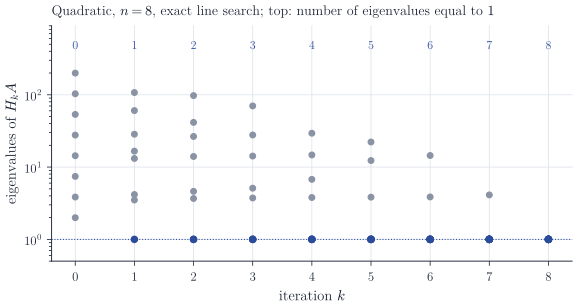
On a strictly convex quadratic \(f(x) = \tfrac12 x^\top A x - b^\top x\), every difference satisfies \(y_k = As_k\), and with exact line searches BFGS has a hereditary property: \(H_k y_j = s_j\) for all \(j < k\), not only for \(j = k-1\). The search directions are then conjugate with respect to \(A\), the method terminates in at most \(n\) steps, and if \(n\) steps are taken, \(H_n = A^{-1}\) (Nocedal and Wright, Chapter 6; the proof is an induction on \(k\) along the lines of the corresponding argument for conjugate gradients). Since \(H_k A s_j = H_k y_j = s_j\), the matrix \(H_kA\) has the eigenvalue \(1\) on the span of \(s_0, \dots, s_{k-1}\), and the approximation is exact on a subspace that grows by one dimension per step. Figure 1 shows this for \(n = 8\). With \(H_0 = I\), BFGS with exact line searches on a quadratic generates the same iterates as conjugate gradients.
Convergence on general functions
Away from quadratics, the guarantees are local and asymptotic. The key result is the characterization of Dennis and Moré: if \(x_k \to x_\star\), \(x_k \neq x_\star\), where \(\nabla f(x_\star) = 0\) and \(\nabla^2 f(x_\star) \succ 0\) and \(\nabla^2 f\) Lipschitz near \(x_\star\), and unit steps are taken eventually, then convergence is superlinear if and only if
\[\frac{\lVert (B_k - \nabla^2 f(x_\star))\, p_k\rVert}{\lVert p_k\rVert} \to 0 .\]The approximation need not converge to the Hessian; it only has to become accurate along the search directions, which is what the secant equation enforces step by step. For BFGS this condition holds under standard assumptions, for instance when the iterates converge to such a minimizer fast enough that \(\sum_k \lVert x_k - x_\star\rVert < \infty\), and the unit step is then eventually accepted by the Wolfe conditions when \(c_1 < 1/2\); for convex \(f\) with bounded level sets, global convergence of BFGS with a Wolfe line search was proved by Powell (1976). Precise statements are in Chapter 6 of Nocedal and Wright and in Dennis and Moré, “Quasi-Newton methods, motivation and theory” (SIAM Review, 1977).
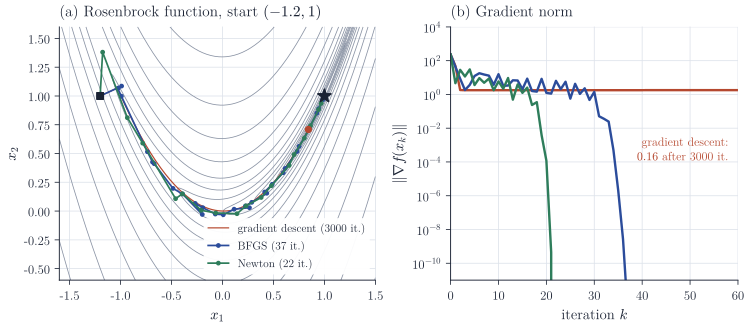
Figure 2 shows the typical picture on the Rosenbrock function. Newton’s method, with a backtracking line search, needs 22 iterations to reach a gradient norm of \(10^{-10}\); BFGS needs 37, without second derivatives; gradient descent with a fixed step crawls along the curved valley and after 3000 iterations has reached only \((0.84, 0.71)\), with gradient norm 0.16. The final iterations of BFGS show the superlinear phase: the gradient norm falls by several orders of magnitude per step.
Limited memory
Storing \(H_k\) costs \(O(n^2)\) memory, which is prohibitive for large \(n\). Unrolling the update shows that \(H_k g\) can be computed from \(H_0\) and the pairs \((s_j, y_j)\) alone. L-BFGS keeps only the most recent \(m\) pairs, typically \(m\) between 3 and 20, and evaluates \(H_k g\) by a two-loop recursion in \(O(mn)\) operations:
def lbfgs_direction(g, S, Y, gamma):
    # H g for the L-BFGS matrix built from the pairs (S[i], Y[i]),
    # oldest first, with initial matrix gamma * I
    q, alphas = g.copy(), []
    for s, y in reversed(list(zip(S, Y))):
        a = (s @ q) / (y @ s); alphas.append(a); q -= a * y
    r = gamma * q
    for (s, y), a in zip(zip(S, Y), reversed(alphas)):
        b = (y @ r) / (y @ s); r += (a - b) * s
    return r            # the search direction is -r
The limited-memory method loses the superlinear rate in general but keeps much of the practical benefit, and with \(\gamma\) set to \(s^\top y / y^\top y\) from the latest pair it is the default optimizer for smooth, unconstrained problems in many statistical and machine-learning libraries, from penalized likelihoods to variational objectives.