Replication on a binomial tree: risk-neutral pricing, early exercise and the Black–Scholes limit
Cox, Ross and Rubinstein (1979) introduced a model in which the stock price moves up or down by a fixed factor in each period. The model is crude as a description of prices, but it contains the whole logic of arbitrage pricing in a form where every step is finite-dimensional linear algebra. A claim can be reproduced exactly by a trading strategy in the stock and a riskless bond; its price is therefore the cost of that strategy, and that cost turns out to be an expectation under a probability measure that has nothing to do with the real chances of an up move. The one-period argument extends by backward induction to many periods and to American options, and as the number of periods grows the tree prices converge to the Black–Scholes prices.
One period
There are two assets and two dates. A bond costs \(1\) at time \(0\) and pays \(R > 0\) at time \(1\). A stock costs \(S_0 > 0\) and is worth \(S_1 = uS_0\) with probability \(p\) or \(S_1 = dS_0\) with probability \(1 - p\), where \(0 < d < u\) and \(0 < p < 1\). A portfolio holds \(\Delta\) shares and \(B\) units of currency in the bond, so its value is \(X_0 = \Delta S_0 + B\) at time \(0\) and \(X_1 = \Delta S_1 + BR\) at time \(1\); negative positions are allowed. An arbitrage is a portfolio with \(X_0 \le 0\), \(X_1 \ge 0\) in both states, and \(X_1 > 0\) in at least one state.
Proposition 1. The one-period model admits no arbitrage if and only if \(d < R < u\). In that case set
\[q = \frac{R - d}{u - d} \in (0, 1).\]A claim paying \(V_u\) in the up state and \(V_d\) in the down state is replicated by the portfolio
\[\Delta = \frac{V_u - V_d}{(u - d) S_0}, \qquad B = \frac{u V_d - d V_u}{(u - d) R},\]whose cost is
\[\begin{equation} V_0 = \frac{1}{R}\bigl\{q V_u + (1 - q) V_d\bigr\}. \label{eq:one-period} \end{equation}\]Any price for the claim other than \(V_0\) creates an arbitrage.
Proof. If \(R \ge u\), sell one share and put \(S_0\) in the bond: \(X_0 = 0\) and \(X_1 = S_0 R - S_1\), which is nonnegative in both states and equals \(S_0(R - d) > 0\) in the down state. If \(R \le d\), the reverse position (borrow \(S_0\), buy one share) has \(X_0 = 0\) and \(X_1 = S_1 - S_0 R \ge 0\), positive in the up state.
Suppose \(d < R < u\). Then \(q \in (0, 1)\) and \(q u + (1 - q) d = R\), so for every portfolio
\[q X_1(\text{up}) + (1 - q) X_1(\text{down}) = \Delta S_0 \{q u + (1 - q) d\} + BR = R X_0 .\]If \(X_1 \ge 0\) in both states and positive in one, the left-hand side is positive because \(q\) and \(1 - q\) are, so \(X_0 > 0\) and there is no arbitrage. The formulas for \(\Delta\) and \(B\) solve the two linear equations \(\Delta u S_0 + BR = V_u\) and \(\Delta d S_0 + BR = V_d\), and the cost identity above, applied to this portfolio, gives \(\eqref{eq:one-period}\). Finally, if the claim trades at \(c > V_0\), selling it, buying the replicating portfolio and putting \(c - V_0\) in the bond costs nothing and pays \((c - V_0) R > 0\) in both states; the case \(c < V_0\) is symmetric.
The real-world probability \(p\) does not appear in the price. Whatever investors believe about \(p\) is already reflected in \(S_0\), and the claim is priced relative to the stock. The number \(q\) is the probability under which the stock earns the riskless return, \(q\, uS_0 + (1 - q)\, dS_0 = RS_0\); it is called the risk-neutral or martingale probability. The hedge ratio \(\Delta\) is a difference quotient of the claim’s payoff with respect to the stock price.
Many periods
Over \(N\) periods, let \(\xi_1, \dots, \xi_N\) take values in \(\{u, d\}\), set \(S_n = S_0 \xi_1 \cdots \xi_n\) and let \(\mathcal F_n = \sigma(\xi_1, \dots, \xi_n)\). Under the real-world measure \(\P\) every one of the \(2^N\) paths has positive probability; nothing else about \(\P\) will matter. A self-financing strategy starts with capital \(X_0\) and holds \(\Delta_n\) shares during period \(n+1\), where \(\Delta_n\) is \(\mathcal F_n\)-measurable, with the rest of the wealth in the bond:
\[X_{n+1} = \Delta_n S_{n+1} + R\,(X_n - \Delta_n S_n).\]Write \(\tilde X_n = R^{-n} X_n\) and \(\tilde S_n = R^{-n} S_n\) for discounted values; then \(\tilde X_{n+1} - \tilde X_n = \Delta_n(\tilde S_{n+1} - \tilde S_n)\). Let \(\mathbb Q\) be the measure under which \(\xi_1, \dots, \xi_N\) are independent with \(\mathbb Q(\xi_j = u) = q\). Since \(qu + (1-q)d = R\),
\[\E_{\mathbb Q}\bigl[\tilde S_{n+1} \mid \mathcal F_n\bigr] = \tilde S_n \,\frac{qu + (1-q)d}{R} = \tilde S_n ,\]so \(\tilde S\) is a \(\mathbb Q\)-martingale, and so is \(\tilde X\) for every self-financing strategy, being a martingale transform of \(\tilde S\) by the predictable process \(\Delta\) (all random variables here take finitely many values, so integrability is automatic). In particular \(X_0 = R^{-N} \E_{\mathbb Q} X_N\), and since \(\mathbb Q\) also charges every path, the argument of Proposition 1 shows that no self-financing strategy is an arbitrage.
Theorem 2. Assume \(d < R < u\), and let \(V_N\) be any \(\mathcal F_N\)-measurable payoff. Define
\[V_n = R^{-(N-n)}\, \E_{\mathbb Q}\bigl[V_N \mid \mathcal F_n\bigr], \qquad n = 0, \dots, N .\]There is a self-financing strategy with \(X_0 = V_0\) and \(X_n = V_n\) for all \(n\); in particular it replicates \(V_N\), and \(V_0 = R^{-N} \E_{\mathbb Q} V_N\) is the only price of the claim that does not create an arbitrage. If \(V_N = g(S_N)\), then \(V_n = v_n(S_n)\), where \(v_N = g\) and
\[v_n(s) = \frac1R\bigl\{q\, v_{n+1}(us) + (1 - q)\, v_{n+1}(ds)\bigr\}, \qquad \Delta_n = \frac{v_{n+1}(uS_n) - v_{n+1}(dS_n)}{(u - d) S_n}.\]Proof. Fix \(n\) and a history \((\xi_1, \dots, \xi_n)\). By the tower property and independence of \(\xi_{n+1}\) from \(\mathcal F_n\) under \(\mathbb Q\), \(V_n = R^{-1}\{q V_{n+1}^{u} + (1 - q) V_{n+1}^{d}\}\), where \(V_{n+1}^{u}\) and \(V_{n+1}^{d}\) are the values of \(V_{n+1}\) after the history is extended by \(u\) and by \(d\). This is a one-period problem with stock price \(S_n\), and Proposition 1 provides \(\Delta_n\), a function of the history, such that a portfolio worth \(V_n\) at time \(n\) is worth \(V_{n+1}\) at time \(n+1\) in both continuations. Starting from \(X_0 = V_0\) and using these \(\Delta_n\), induction gives \(X_n = V_n\) for every \(n\). If the claim traded at a price other than \(V_0\), combining it with this strategy and the bond would give an arbitrage as in Proposition 1. Conversely, if the claim is traded at the prices \(V_n\), its discounted price \(R^{-n} V_n = R^{-N}\E_{\mathbb Q}[V_N \mid \mathcal F_n]\) is a \(\mathbb Q\)-martingale, so every self-financing strategy in the stock, the bond and the claim has a discounted value that is a \(\mathbb Q\)-martingale, and the argument before the theorem excludes arbitrage. When \(V_N = g(S_N)\), the recursion for \(v_n\) follows by backward induction because \(S_{n+1} \in \{uS_n, dS_n\}\).
For a European call, \(g(s) = (s - K)^+\), the expectation can be written in closed form. Let \(a\) be the smallest integer \(k\) with \(S_0 u^k d^{N-k} > K\) and let \(\Psi(a; N, \pi)\) be the probability that a \(\mathrm{Binomial}(N, \pi)\) variable is at least \(a\). With \(\hat q = qu/R\), which lies in \((0,1)\) because \(qu/R + (1-q)d/R = 1\),
\[C_0 = R^{-N} \sum_{k = a}^{N} \binom Nk q^k (1-q)^{N-k} \bigl(S_0 u^k d^{N-k} - K\bigr) = S_0\, \Psi(a; N, \hat q) - K R^{-N}\, \Psi(a; N, q),\]where the first term uses \(R^{-N} q^k (1-q)^{N-k} u^k d^{N-k} = \hat q^{\,k} (1 - \hat q)^{N-k}\). The formula has the same shape as the Black–Scholes formula, with binomial tail probabilities in place of normal ones.
American options
An American option with payoff function \(g\) can be exercised at any date \(n \in \{0, \dots, N\}\) chosen by the holder on the basis of the information available, that is, at a stopping time of \((\mathcal F_n)\). The pricing recursion compares the value of exercising with the value of waiting:
\[v_N = g, \qquad v_n(s) = \max\Bigl\{ g(s),\ \frac1R\bigl\{q\, v_{n+1}(us) + (1 - q)\, v_{n+1}(ds)\bigr\} \Bigr\}.\]Theorem 3. Let \(Z_n = R^{-n} g(S_n)\) and \(U_n = R^{-n} v_n(S_n)\), and let \(\mathcal T\) be the set of stopping times with values in \(\{0, \dots, N\}\). Then \(U\) is the smallest \(\mathbb Q\)-supermartingale that dominates \(Z\), and
\[v_0(S_0) = U_0 = \max_{\tau \in \mathcal T} \E_{\mathbb Q} Z_\tau ,\]with the maximum attained at \(\tau^* = \min\{n : v_n(S_n) = g(S_n)\}\).
Proof. By construction \(U_n \ge Z_n\) and \(U_n \ge \E_{\mathbb Q}[U_{n+1} \mid \mathcal F_n]\), the latter being \(R^{-n}\) times the continuation value. For \(\tau \in \mathcal T\), optional stopping for a supermartingale and a bounded stopping time gives \(\E_{\mathbb Q} Z_\tau \le \E_{\mathbb Q} U_\tau \le U_0\). The time \(\tau^*\) is a stopping time bounded by \(N\), since \(v_N = g\). On \(\{\tau^* > n\}\) the maximum in the recursion is attained by the continuation value, so \(U_n = \E_{\mathbb Q}[U_{n+1} \mid \mathcal F_n]\) there. Hence the increments \(U_{(n+1)\wedge\tau^*} - U_{n\wedge\tau^*} = \mathbf 1\{\tau^* > n\}(U_{n+1} - U_n)\) have zero conditional mean, the stopped process is a martingale, and \(U_0 = \E_{\mathbb Q} U_{\tau^*} = \E_{\mathbb Q} Z_{\tau^*}\). If \(Y\) is another supermartingale with \(Y \ge Z\), then \(Y_N \ge Z_N = U_N\), and if \(Y_{n+1} \ge U_{n+1}\) then \(Y_n \ge \max\{Z_n, \E_{\mathbb Q}[Y_{n+1} \mid \mathcal F_n]\} \ge U_n\); backward induction gives \(Y \ge U\).
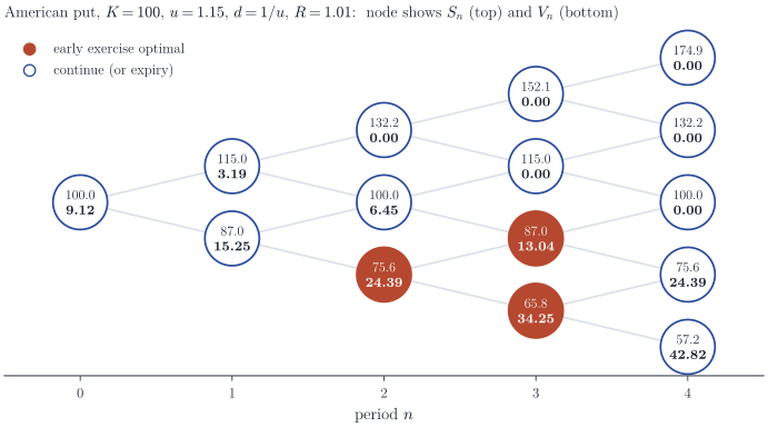
The financial content is the following. The seller who receives \(v_0(S_0)\) can hedge the continuation value at each node with the \(\Delta_n\) of Theorem 2, consuming the difference whenever \(v_n\) exceeds the continuation value; the portfolio is then worth \(v_n(S_n) \ge g(S_n)\) at every date, so any exercise can be honoured. The holder who exercises at \(\tau^*\) receives a payoff whose value is exactly \(v_0(S_0)\). Figure 1 shows the recursion for a put on a four-period tree.
For a call on a stock that pays no dividends, early exercise is never strictly better when \(R \ge 1\). Indeed, by the conditional Jensen inequality for the convex function \(x \mapsto (x - K)^+\),
\[\E_{\mathbb Q}\bigl[Z_{n+1} \mid \mathcal F_n\bigr] \ge R^{-(n+1)}\bigl(\E_{\mathbb Q}[S_{n+1} \mid \mathcal F_n] - K\bigr)^+ = R^{-n}\bigl(S_n - K/R\bigr)^+ \ge R^{-n} (S_n - K)^+ = Z_n ,\]so \(Z\) is a \(\mathbb Q\)-submartingale, optional stopping gives \(\E_{\mathbb Q} Z_\tau \le \E_{\mathbb Q} Z_N\) for every \(\tau \in \mathcal T\), and the American call is worth the same as the European one. For the put the same computation gives only the lower bound \(R^{-n}(K/R - S_n)^+\), which is smaller than \(Z_n\) when \(R > 1\) and \(S_n < K\), and early exercise can indeed be optimal, as in Figure 1.
The recursion is a few lines of code:
import numpy as np

def american_put(S0, K, u, d, R, N):
    q = (R - d) / (u - d)
    k = np.arange(N + 1)
    v = np.maximum(K - S0 * u**k * d**(N - k), 0.0)   # time N
    for n in range(N - 1, -1, -1):
        k = np.arange(n + 1)
        cont = (q * v[1:n + 2] + (1 - q) * v[:n + 1]) / R
        v = np.maximum(K - S0 * u**k * d**(n - k), cont)
    return v[0]
With the parameters of Figure 1, american_put(100, 100, 1.15, 1/1.15, 1.01, 4) returns \(9.12\).
The Black–Scholes limit
Fix a maturity \(T > 0\), a continuously compounded rate \(r \in \R\) and a volatility \(\sigma > 0\). With \(N\) periods of length \(h = T/N\), take
\[u_N = e^{\sigma\sqrt h}, \qquad d_N = e^{-\sigma\sqrt h}, \qquad R_N = e^{rh},\]so that \(R_N^{N} = e^{rT}\) exactly. Since \(rh = o(\sigma\sqrt h)\), the condition \(d_N < R_N < u_N\) holds for all large \(N\). Expanding numerator and denominator of \(q_N = (e^{rh} - e^{-\sigma\sqrt h})/(e^{\sigma\sqrt h} - e^{-\sigma\sqrt h})\) in powers of \(\sqrt h\),
\[\begin{equation} \begin{aligned} q_N &= \frac{\sigma\sqrt h + (r - \sigma^2/2)h + \sigma^3 h^{3/2}/6 + O(h^2)}{2\sigma\sqrt h + \sigma^3 h^{3/2}/3 + O(h^{5/2})} \\ &= \frac12 + \frac{r - \sigma^2/2}{2\sigma}\sqrt h + O(h^{3/2}). \end{aligned} \label{eq:qN} \end{equation}\]Theorem 4. Under \(\mathbb Q_N\), \(\log(S_N/S_0) \Rightarrow \mathcal N\bigl((r - \sigma^2/2)T,\ \sigma^2 T\bigr)\) as \(N \to \infty\). Consequently the European put and call prices on the \(N\)-period tree converge to
\[P_{\mathrm{BS}} = K e^{-rT} \Phi(-d_2) - S_0 \Phi(-d_1), \qquad C_{\mathrm{BS}} = S_0 \Phi(d_1) - K e^{-rT} \Phi(d_2),\]where \(d_{1,2} = \{\log(S_0/K) + (r \pm \sigma^2/2)T\}/(\sigma\sqrt T)\) and \(\Phi\) is the standard normal distribution function.
Proof. Write \(\log(S_N/S_0) = \sum_{j=1}^N Y_{N,j}\), where under \(\mathbb Q_N\) the \(Y_{N,j}\) are independent and equal \(+\sigma\sqrt h\) with probability \(q_N\) and \(-\sigma\sqrt h\) otherwise. By \(\eqref{eq:qN}\), the mean is
\[N\sigma\sqrt h\,(2q_N - 1) = N\sigma\sqrt h \Bigl\{\frac{r - \sigma^2/2}{\sigma}\sqrt h + O(h^{3/2})\Bigr\} = (r - \sigma^2/2)T + O(h),\]and the variance is \(N\sigma^2 h \cdot 4q_N(1 - q_N) = \sigma^2 T\{1 - (2q_N - 1)^2\} \to \sigma^2 T\). The centred summands are bounded by \(2\sigma\sqrt h\), so for every \(\varepsilon > 0\) the Lindeberg sum \(\sum_j \E[(Y_{N,j} - \E Y_{N,j})^2 \mathbf 1\{\abs{Y_{N,j} - \E Y_{N,j}} > \varepsilon\}]\) is zero as soon as \(2\sigma\sqrt h < \varepsilon\). The Lindeberg–Feller theorem and Slutsky’s lemma give the stated limit \(Z \sim \mathcal N((r - \sigma^2/2)T, \sigma^2 T)\).
The put payoff \(x \mapsto (K - S_0 e^x)^+\) is bounded and continuous, so weak convergence gives \(P_N = e^{-rT}\E_{\mathbb Q_N}(K - S_N)^+ \to e^{-rT}\E(K - S_0 e^{Z})^+\). For the call, the identity \((s - K)^+ - (K - s)^+ = s - K\) and the martingale property \(\E_{\mathbb Q_N} S_N = R_N^N S_0\) give put–call parity on the tree, \(C_N - P_N = S_0 - Ke^{-rT}\), for every \(N\); the same identity holds for the limits. It remains to evaluate the Gaussian expectations. With \(m = (r - \sigma^2/2)T\), \(s = \sigma\sqrt T\) and \(c = \log(K/S_0)\), completing the square gives \(\E[e^Z \mathbf 1\{Z > c\}] = e^{m + s^2/2}\Phi((m + s^2 - c)/s) = e^{rT}\Phi(d_1)\) and \(\P(Z > c) = \Phi((m - c)/s) = \Phi(d_2)\), so \(e^{-rT}\E(S_0 e^Z - K)^+ = C_{\mathrm{BS}}\), and parity gives \(P_{\mathrm{BS}}\).
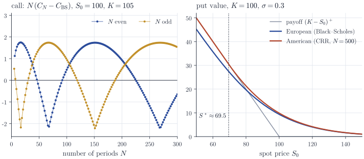
The convergence is not monotone. The left panel of Figure 2 shows that the error of the call price is of order \(1/N\), with a coefficient that differs between even and odd \(N\) and oscillates slowly as \(N\) grows. The source is the position of \(\log K\) relative to the lattice of terminal log-prices, which changes with \(N\). Practical implementations therefore either average consecutive \(N\), smooth the payoff at the last step, or place the strike on a node.
Remarks
The American put prices on the tree also converge as \(N \to \infty\), to the value of the corresponding optimal stopping problem for geometric Brownian motion, but the proof is more delicate than Theorem 4 and is not given here. Unlike the European put, the American put has no closed-form price, and the tree remains a standard way of computing it together with its exercise boundary.
The parametrization \(u_N = 1/d_N = e^{\sigma\sqrt h}\) is one choice among several. The proof of Theorem 4 applies to any choice whose one-period log-returns are bounded by a multiple of \(\sqrt h\) and whose risk-neutral mean and variance equal \((r - \sigma^2/2)h\) and \(\sigma^2 h\) up to \(o(h)\). Expectations under \(\mathbb Q\) describe prices, not forecasts: the drift of the stock under \(\P\) never entered the argument, and it is replaced by the riskless rate in every formula.
The original paper is Cox, Ross and Rubinstein, Option pricing: a simplified approach (J. Financial Economics, 1979). Shreve, Stochastic Calculus for Finance I: The Binomial Asset Pricing Model (Springer, 2004), develops the model in detail, including American options; Föllmer and Schied, Stochastic Finance (de Gruyter), treats the discrete-time theory of arbitrage and optimal stopping in general.