From two uniforms to two Gaussians: the Box–Muller transform and the polar method
Every call to a normal random number generator ends in arithmetic on uniform pseudorandom numbers. The generic route is inversion: if \(U \sim \mathrm{Uniform}(0,1)\) and \(F\) is a continuous distribution function, then \(F^{-1}(U)\) has distribution \(F\). For the standard normal this requires \(\Phi^{-1}\), which has no closed form; it can be evaluated to machine precision by rational approximations, but the approximation is the whole difficulty. The Box–Muller transform avoids \(\Phi^{-1}\) entirely by generating two normals at once. In two dimensions the Gaussian becomes simple, because its density depends only on the distance to the origin.
Throughout, \(U_1, U_2\) are independent \(\mathrm{Uniform}(0,1)\) random variables and \(\phi_2(z) = (2\pi)^{-1} e^{-\norm{z}^2/2}\) is the standard bivariate normal density on \(\R^2\).
The idea in polar coordinates
Suppose \(Z = (Z_1, Z_2)\) already has density \(\phi_2\), and write it in polar form \(Z = (R\cos\Theta, R\sin\Theta)\). Because \(\phi_2\) is invariant under rotations, the angle \(\Theta\) should be uniform on \((0, 2\pi)\) and independent of \(R\). The radius satisfies \(R^2 = Z_1^2 + Z_2^2 \sim \chi^2_2\), and a \(\chi^2_2\) variable is exponential with mean \(2\): \(\P(R^2 > s) = e^{-s/2}\). Each of these two laws is easy to simulate by inversion. An angle is \(2\pi U_2\), and an exponential with mean 2 is \(-2\log U_1\), since \(\P(-2\log U_1 > s) = \P(U_1 < e^{-s/2}) = e^{-s/2}\). Reversing the argument suggests
\[\begin{equation} Z_1 = \sqrt{-2\log U_1}\,\cos(2\pi U_2), \qquad Z_2 = \sqrt{-2\log U_1}\,\sin(2\pi U_2). \label{eq:bm} \end{equation}\]The heuristic uses facts about \(Z\) that we are trying to produce, so it needs a direct proof.
Proposition 1 (Box–Muller). The pair \((Z_1, Z_2)\) defined by \(\eqref{eq:bm}\) consists of two independent \(N(0,1)\) random variables.
Proof. Put \(R = \sqrt{-2\log U_1}\) and \(\Theta = 2\pi U_2\); they are independent because \(U_1\) and \(U_2\) are. From \(\P(R > r) = \P(U_1 < e^{-r^2/2}) = e^{-r^2/2}\) for \(r > 0\), the variable \(R\) has density \(r e^{-r^2/2}\) on \((0, \infty)\), so \((R, \Theta)\) has density
\[g(r, \theta) = \frac{1}{2\pi}\, r\, e^{-r^2/2}, \qquad (r,\theta) \in (0,\infty) \times (0, 2\pi).\]The polar map \(T(r, \theta) = (r\cos\theta, r\sin\theta)\) is a continuously differentiable bijection from \((0,\infty)\times(0,2\pi)\) onto \(\R^2 \setminus L\), where \(L = \{(x, 0) : x \ge 0\}\), and its Jacobian determinant is \(r\). Since \(Z = T(R, \Theta)\) never lies in \(L\), and \(L\) has Lebesgue measure zero, the change of variables formula gives, for every Borel set \(B \subseteq \R^2\),
\[\P(Z \in B) = \int_{(0,\infty)\times(0,2\pi)} \mathbf 1_B\bigl(T(r,\theta)\bigr)\, \phi_2\bigl(T(r,\theta)\bigr)\, r \,\dd r\,\dd\theta = \int_B \phi_2(z)\,\dd z,\]where we used \(g(r,\theta) = \phi_2(T(r,\theta))\, r\). Thus \(Z\) has density \(\phi_2(z) = (2\pi)^{-1/2}e^{-z_1^2/2}\cdot(2\pi)^{-1/2}e^{-z_2^2/2}\), which factorizes into two standard normal densities.
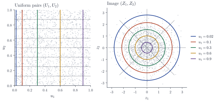
Figure 1 shows the transform as a map of the unit square onto the plane. A vertical line \(u_1 = a\) becomes the circle of radius \(\sqrt{-2\log a}\), and a horizontal line \(u_2 = b\) becomes the ray at angle \(2\pi b\). The strip \(u_1 < 0.02\), two percent of the square, is spread over the whole exterior of the circle of radius \(\sqrt{-2\log 0.02} \approx 2.80\); the strip \(u_1 > 0.9\) is squeezed into a disc of radius \(0.46\) around the origin. The tails of the normal come from a thin sliver of the square near \(u_1 = 0\).
Two practical details
The formula \(\eqref{eq:bm}\) needs \(U_1 > 0\). Many generators return values in \([0, 1)\), in which case one should use \(1 - U_1\) instead, which lies in \((0, 1]\) and has the same distribution. The same observation bounds the output. If the generator returns multiples of \(2^{-53}\), the smallest positive value of \(U_1\) is \(2^{-53}\), so
\[\sqrt{Z_1^2 + Z_2^2} = R \le \sqrt{2 \cdot 53 \log 2} \approx 8.57 .\]Under the exact normal law \(\P(R > 8.57) \approx 2^{-53} \approx 1.1 \times 10^{-16}\), so this truncation is invisible in any simulation of practical size; it is exactly the probability of the smallest atom of the discretized uniform.
The second detail concerns the input pairs. The map \(\eqref{eq:bm}\) is smooth, so any regular structure in consecutive pairs \((U_1, U_2)\), such as the lattice structure produced by simple linear congruential generators, is transported to a visible pattern in the plane. Proposition 1 assumes genuinely independent uniforms, and the quality of the output can be no better than the quality of the input pairs.
Avoiding trigonometric functions: the polar method
Each Box–Muller pair costs one logarithm, one square root, a sine and a cosine. Marsaglia’s polar method removes the trigonometric functions by generating the point \((\cos\Theta, \sin\Theta)\) geometrically: a point drawn uniformly from the unit disc has a uniformly distributed direction, and its squared radius turns out to be a uniform variable that can play the role of \(U_1\).
The algorithm is as follows. Draw \(V_1, V_2\) independent \(\mathrm{Uniform}(-1, 1)\) and set \(S = V_1^2 + V_2^2\). If \(S \ge 1\) or \(S = 0\), discard the pair and draw again. Otherwise return
\[\begin{equation} Z_1 = V_1\sqrt{\frac{-2\log S}{S}}, \qquad Z_2 = V_2\sqrt{\frac{-2\log S}{S}} . \label{eq:polar} \end{equation}\]Two facts are needed: the accepted point is uniform on the punctured disc \(D = \{v : 0 < \norm{v} < 1\}\), and a uniform point on \(D\) yields normals through \(\eqref{eq:polar}\).
Lemma 2 (Rejection). Let \(W_1, W_2, \dots\) be independent and uniform on the square \(Q = (-1,1)^2\), let \(\tau = \min\{k : W_k \in D\}\), and let \(p = \lambda(D)/\lambda(Q) = \pi/4\), where \(\lambda\) is Lebesgue measure. Then \(\tau\) is geometric with success probability \(p\), and \(W_\tau\) is uniform on \(D\).
Proof. The events \(\{W_k \in D\}\) are independent with probability \(p\), which gives the law of \(\tau\) and shows \(\tau < \infty\) almost surely. For a Borel set \(B\), by independence,
\[\begin{aligned} \P(W_\tau \in B) &= \sum_{k \ge 1} \P(W_1 \notin D, \dots, W_{k-1} \notin D,\ W_k \in B \cap D) \\ &= \sum_{k\ge1} (1-p)^{k-1}\, \frac{\lambda(B \cap D)}{\lambda(Q)} = \frac{\lambda(B\cap D)}{p\,\lambda(Q)} , \end{aligned}\]and \(p\,\lambda(Q) = \lambda(D)\).
Proposition 3 (Polar method). If \(V = (V_1, V_2)\) is uniform on \(D\) and \(S = \norm{V}^2\), then \(S \sim \mathrm{Uniform}(0,1)\), the direction \(V/\sqrt{S}\) is uniform on the unit circle, and the two are independent. Consequently \((Z_1, Z_2)\) in \(\eqref{eq:polar}\) are independent \(N(0,1)\).
Proof. Write \(V = (\rho\cos\varphi, \rho\sin\varphi)\) with \(\rho \in (0,1)\) and \(\varphi \in [0, 2\pi)\). For \(s \in (0,1]\) and an interval \(A \subseteq [0, 2\pi)\) of length \(\abs{A}\), the set \(\{\rho^2 \le s, \varphi \in A\}\) is a sector of the disc of radius \(\sqrt s\) with area \(s\abs{A}/2\). Dividing by \(\lambda(D) = \pi\),
\[\P(S \le s,\ \varphi \in A) = s \cdot \frac{\abs{A}}{2\pi} .\]These sets form a \(\pi\)-system generating the Borel sets of \((0,1]\times[0,2\pi)\), so the joint law of \((S, \varphi)\) is the product of \(\mathrm{Uniform}(0,1)\) and \(\mathrm{Uniform}(0, 2\pi)\). Now \(V/\sqrt S = (\cos\varphi, \sin\varphi)\), and \(\eqref{eq:polar}\) reads \(Z = \sqrt{-2\log S}\,(\cos\varphi, \sin\varphi)\). This is \(\eqref{eq:bm}\) with \(U_1 = S\) and \(U_2 = \varphi/(2\pi)\), which are independent uniforms, so Proposition 1 applies.
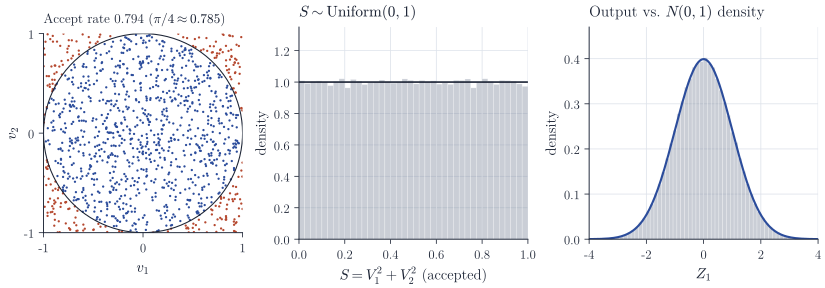
The price of avoiding sine and cosine is the rejection step. By Lemma 2 the expected number of trials per accepted pair is \(4/\pi \approx 1.27\), that is, about \(8/\pi \approx 2.55\) uniforms per pair of normals instead of two. Figure 2 shows the rejected corners of the square, the uniformity of \(S\) among accepted points, and the agreement of the output with the standard normal density.
A minimal implementation, vectorized by oversampling, takes a few lines:
import numpy as np

def polar_normals(n, rng):
    """Return 2*n independent N(0,1) draws by Marsaglia's polar method."""
    out = []
    while sum(len(z) for z in out) < 2 * n:
        v = rng.uniform(-1.0, 1.0, size=(n, 2))
        s = (v ** 2).sum(axis=1)
        ok = (s > 0) & (s < 1)
        v, s = v[ok], s[ok]
        out.append((v * np.sqrt(-2.0 * np.log(s) / s)[:, None]).ravel())
    return np.concatenate(out)[: 2 * n]
Remarks
Both methods are exact: given independent uniforms, the output has exactly the normal law, with no approximation beyond floating point arithmetic. This distinguishes them from inversion, whose accuracy rests on the approximation of \(\Phi^{-1}\), and from older recipes such as summing twelve uniforms and subtracting six, which matches the normal mean and variance (and, by symmetry, the third moment) but has bounded support and the wrong fourth moment. Current software uses a variety of methods. R’s default normal generator is inversion with a high-accuracy approximation of \(\Phi^{-1}\); NumPy’s legacy RandomState uses the polar method, and its newer Generator interface uses a ziggurat algorithm, a refined rejection scheme in which the great majority of draws need only a table lookup, a multiplication and a comparison.
Normal vectors with mean \(\mu\) and covariance \(\Sigma\) follow by an affine map: if \(Z\) has independent \(N(0,1)\) entries and \(LL^\top = \Sigma\), for instance with \(L\) the Cholesky factor, then \(\mu + LZ \sim N(\mu, \Sigma)\).
The original sources are G. E. P. Box and M. E. Muller, “A note on the generation of random normal deviates” (Annals of Mathematical Statistics, 1958), and G. Marsaglia and T. A. Bray, “A convenient method for generating normal variables” (SIAM Review, 1964). L. Devroye’s Non-Uniform Random Variate Generation treats these and many other methods in detail.