From Brownian motion to Itô processes: drift, diffusion and quadratic variation

October 12, 2026Stochastic processes and time series

Continuous-time models in finance, physics and statistics are usually written as a deterministic trend plus a noise term, \(dX_t = \mu_t\,dt + \sigma_t\,dW_t\). The noise is driven by a Wiener process \(W\), and much of what is unusual about such models comes from one property of \(W\): over a short interval of length \(\Delta\), its increment has size of order \(\sqrt\Delta\), far larger than the \(\Delta\) contributed by the trend. The precise form of this property is the quadratic variation of \(W\); it explains why the stochastic integral needs its own construction, and it has a sharp statistical consequence: on a fixed time window the noise level can be recovered exactly from a path, while the trend cannot.

All processes live on a probability space \((\Omega, \mathcal F, \P)\) with a filtration \((\mathcal F_t)_{t\ge0}\).

The Wiener process

A heuristic first. Let \(\xi_1, \xi_2, \dots\) be independent with mean zero and variance one, and consider a random walk that takes a step every \(\Delta\) time units. For the walk to have a nondegenerate limit as \(\Delta \to 0\), its variance at time \(t\), which is \((t/\Delta) \cdot \mathrm{(step\ size)}^2\), must stay of order \(t\). Steps must therefore have size \(\sqrt\Delta\), and by the central limit theorem the position at time \(t\) is approximately \(N(0, t)\), independently of the law of the \(\xi_i\). The limit object is characterized as follows.

A (standard) Wiener process, or Brownian motion, with respect to \((\mathcal F_t)\) is an adapted process \(W = (W_t)_{t\ge0}\) such that

1. \(W_0 = 0\) and \(t \mapsto W_t(\omega)\) is continuous for every \(\omega\);
2. for \(0 \le s < t\), the increment \(W_t - W_s\) is independent of \(\mathcal F_s\) and has the \(N(0, t - s)\) distribution.

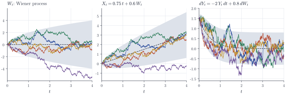
Existence is a theorem (due to Wiener; Lévy’s construction by successive interpolation is a short proof), and the finite-dimensional distributions are determined by the definition: \((W_{t_1}, \dots, W_{t_k})\) is a centred Gaussian vector with \(\Cov(W_s, W_t) = \min(s,t)\). Property 2 implies that \(W\) is a martingale and that \(W_t^2 - t\) is a martingale. The left panel of Figure 1 shows five paths together with the band \(\pm2\sqrt t\).

Figure 1. Five simulated paths of each process, driven by the same Brownian increments, with the mean (dashed) and the band of two standard deviations around it (shaded). Left: the Wiener process, whose spread grows like $\sqrt t$. Middle: Brownian motion with drift $a = 0.75$ and scale $b = 0.6$; the trend $at$ eventually dominates the fluctuations of size $b\sqrt t$. Right: an Ornstein–Uhlenbeck process started at $1.5$, an Itô process whose drift pulls it back to zero.

Quadratic variation

For a partition \(\pi = \{0 = t_0 < t_1 < \dots < t_n = t\}\) of \([0, t]\) write \(\Delta_i W = W_{t_i} - W_{t_{i-1}}\), \(\Delta t_i = t_i - t_{i-1}\), and \(\abs{\pi} = \max_i \Delta t_i\) for the mesh.

Proposition 1. Let \(\pi_n\) be partitions of \([0,t]\) with \(\abs{\pi_n} \to 0\). Then

\[Q_n = \sum_{i} (\Delta_i W)^2 \longrightarrow t \quad \text{in } L^2 .\]

If moreover \(\sum_n \abs{\pi_n} < \infty\), the convergence also holds almost surely.

Proof. The summands \((\Delta_i W)^2 - \Delta t_i\) are independent with mean zero, and \(\Var\{(\Delta_i W)^2\} = 2(\Delta t_i)^2\) because \(\E Z^4 = 3\) for \(Z \sim N(0,1)\). Hence

\[\E(Q_n - t)^2 = \sum_i \Var\{(\Delta_i W)^2\} = 2\sum_i (\Delta t_i)^2 \le 2t\,\abs{\pi_n} \to 0 .\]

Under the summability condition, Chebyshev’s inequality gives \(\sum_n \P(\abs{Q_n - t} > \varepsilon) \le \varepsilon^{-2}\sum_n 2t\abs{\pi_n} < \infty\) for every \(\varepsilon > 0\), and the first Borel–Cantelli lemma yields almost sure convergence.

A smooth function \(f\) behaves differently: \(\sum_i (\Delta_i f)^2 \le \max_i\abs{\Delta_i f}\cdot\sum_i\abs{\Delta_i f}\), which tends to zero because the first factor does and the second is bounded by the total variation of \(f\). The same inequality turns Proposition 1 into a statement about the roughness of Brownian paths.

Corollary 2. For every \(t > 0\), almost every Brownian path has infinite total variation on \([0, t]\).

Proof. Take dyadic partitions \(\pi_n\) of \([0,t]\) with mesh \(t2^{-n}\), so that \(Q_n \to t\) almost surely. Each path is uniformly continuous on \([0,t]\), so \(\max_i \abs{\Delta_i W} \to 0\). On the event that the total variation \(V\) is finite, \(Q_n \le \max_i\abs{\Delta_i W}\cdot V \to 0\), which is compatible with \(Q_n \to t > 0\) only on a null set.

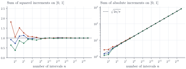
Figure 2 shows both sums along dyadic partitions of \([0,1]\). The sum of squares settles at \(1\); the sum of absolute increments grows like \(\sqrt{2n/\pi}\), since \(\E\abs{\Delta_i W} = \sqrt{2\Delta t_i/\pi}\). Corollary 2 is the reason why \(\int \sigma_s\,dW_s\) cannot be defined path by path as a Riemann–Stieltjes integral, and why a separate construction is needed below.

Figure 2. For three Brownian paths on $[0,1]$ and dyadic partitions with $n = 2^2, \dots, 2^{20}$ intervals: the sum of squared increments (left) converges to $t = 1$, while the sum of absolute increments (right, log scale) diverges along $\sqrt{2n/\pi}$.

Brownian motion with drift

The simplest model with both a trend and noise is the generalized Wiener process

\[X_t = x_0 + a\,t + b\,W_t, \qquad a \in \R,\ b > 0,\]

or \(dX_t = a\,dt + b\,dW_t\). Its increments \(X_t - X_s \sim N\bigl(a(t-s), b^2(t-s)\bigr)\) are independent of \(\mathcal F_s\). Over a short interval of length \(\Delta\) the drift moves the process by \(a\Delta\) and the noise by an amount of order \(b\sqrt\Delta\); over a long interval the order is reversed. The middle panel of Figure 1 shows paths that wander like Brownian motion at short range and follow the line \(x_0 + at\) at long range.

This difference of scales has a sharp statistical form. Suppose the path of \(X\) is observed on \([0, T]\).

Proposition 3. Let \(\pi_n\) be partitions of \([0, T]\) with \(\abs{\pi_n} \to 0\).

1. The realized variance \(\sum_i (\Delta_i X)^2\) converges to \(b^2 T\) in \(L^2\). In particular, for every \(T > 0\) there is a measurable functional of the path on \([0, T]\), the same for all values of \(a\) and \(b\), that equals \(b^2\) almost surely.
2. The estimator \(\hat a_T = (X_T - x_0)/T\) has the \(N(a, b^2/T)\) distribution, whatever the sampling scheme. As \(T \to \infty\), \(\hat a_T \to a\) almost surely.

Proof. For part 1 expand \(\Delta_i X = a\Delta t_i + b\Delta_i W\):

\[\sum_i (\Delta_i X)^2 = b^2\sum_i(\Delta_i W)^2 + 2ab\sum_i \Delta t_i\,\Delta_i W + a^2\sum_i(\Delta t_i)^2 .\]

The first term tends to \(b^2T\) in \(L^2\) by Proposition 1. The second has mean zero and variance \(4a^2b^2\sum_i(\Delta t_i)^3 \le 4a^2b^2T\abs{\pi_n}^2\), and the third is at most \(a^2T\abs{\pi_n}\). Adding the three bounds, \(\E\bigl(\sum_i(\Delta_i X)^2 - b^2T\bigr)^2 \le C(a,b,T)\,\abs{\pi_n}\) for \(\abs{\pi_n} \le 1\). Along a subsequence with \(\sum_k \abs{\pi_{n_k}} < \infty\), which does not depend on \(a\) or \(b\), Chebyshev’s inequality and the Borel–Cantelli lemma give almost sure convergence, so \(\limsup_k \sum_i(\Delta_i X)^2/T\) along \(\pi_{n_k}\) is the required functional.

For part 2, \(\hat a_T = a + bW_T/T\) and \(W_T/T \sim N(0, 1/T)\). For the almost sure limit we show \(W_t/t \to 0\). By the strong law of large numbers applied to the independent standard normal increments \(W_k - W_{k-1}\), \(W_n/n \to 0\) along integers. Let \(M_n = \sup_{s\in[n, n+1]}\abs{W_s - W_n}\); the \(M_n\) are identically distributed, and \(\E M_0 < \infty\) because, by the reflection principle, \(\sup_{s\le1}W_s\) has the law of \(\abs{W_1}\), and \(M_0 \le \sup_{s\le1}W_s + \sup_{s\le1}(-W_s)\). For \(\varepsilon > 0\),

\[\sum_{n\ge1}\P(M_n > \varepsilon n) = \sum_{n\ge1}\P(M_0/\varepsilon > n) \le \E M_0/\varepsilon < \infty,\]

so by Borel–Cantelli \(M_n \le \varepsilon n\) for all large \(n\), almost surely. For \(t \in [n, n+1]\) we have \(\abs{W_t}/t \le (\abs{W_n} + M_n)/n\), whose upper limit is at most \(\varepsilon\).

Sampling the path more finely on a fixed window pins down \(b\) exactly but leaves the uncertainty about \(a\) at \(b/\sqrt T\), and no use of the path can do better. By Girsanov’s theorem the law of \((X_s)_{s\le T}\) under drift \(a\) has density \(\exp\{a(X_T - x_0)/b^2 - a^2T/(2b^2)\}\) with respect to its law under drift \(0\), so \(X_T\) is sufficient for \(a\) (with \(b\) known), and \(\hat a_T\) is the maximum likelihood estimator and the minimum-variance unbiased estimator. Only a longer window helps. This is the continuous-time version of the familiar observation that volatilities can be estimated from high-frequency data much more precisely than expected returns.

Itô processes

Allowing the drift and the noise intensity to vary with time and with the state gives the class of Itô processes. To define them we need \(\int_0^t \sigma_s\,dW_s\) for random integrands. Call \(\sigma\) simple if \(\sigma_s = \xi_{i}\) for \(s \in (t_{i-1}, t_i]\), where \(0 = t_0 < \dots < t_n\) is deterministic and each \(\xi_i\) is \(\mathcal F_{t_{i-1}}\)-measurable and square integrable. For such \(\sigma\) set

\[\int_0^{t_n}\sigma_s\,dW_s = \sum_{i=1}^n \xi_i\,\Delta_i W .\]

The integrand is evaluated at the left endpoint of each interval, before the increment it multiplies is revealed.

Lemma 4 (Itô isometry for simple integrands). For simple \(\sigma\) as above,

\[\E\Bigl(\sum_{i=1}^n \xi_i\,\Delta_i W\Bigr) = 0, \qquad \E\Bigl(\sum_{i=1}^n \xi_i\,\Delta_i W\Bigr)^2 = \E\int_0^{t_n}\sigma_s^2\,ds ,\]

and both quantities are finite.

Proof. Since \(\Delta_i W\) is independent of \(\mathcal F_{t_{i-1}}\) with mean zero and variance \(\Delta t_i\), conditioning on \(\mathcal F_{t_{i-1}}\) gives \(\E[\xi_i\Delta_i W] = 0\) and \(\E[\xi_i^2(\Delta_i W)^2] = \E[\xi_i^2]\,\Delta t_i\). For \(i < j\), the variable \(\xi_i\xi_j\Delta_i W\) is \(\mathcal F_{t_{j-1}}\)-measurable and integrable (by Cauchy–Schwarz and independence of \(\Delta_i W\) from \(\xi_i\)), so conditioning on \(\mathcal F_{t_{j-1}}\) gives \(\E[\xi_i\xi_j\Delta_i W\,\Delta_j W] = 0\). Summing, \(\E(\sum_i\xi_i\Delta_i W)^2 = \sum_i\E[\xi_i^2]\Delta t_i\), which is the right-hand side.

Thus, on simple integrands, \(\sigma \mapsto \int\sigma_s\,dW_s\) is a linear isometry from a subspace of \(L^2(\Omega\times[0,t])\) into \(L^2(\Omega)\). Simple processes are dense in the space of progressively measurable \(\sigma\) with \(\E\int_0^t\sigma_s^2\,ds < \infty\), so the integral extends uniquely to that space, keeping mean zero and the isometry. Further localization extends it to integrands with \(\int_0^t\sigma_s^2\,ds < \infty\) almost surely. The details are in the references below.

An Itô process is a process of the form

\[X_t = X_0 + \int_0^t \mu_s\,ds + \int_0^t \sigma_s\,dW_s,\]

with \(X_0\) being \(\mathcal F_0\)-measurable, \(\mu\) and \(\sigma\) progressively measurable, \(\int_0^t\abs{\mu_s}\,ds < \infty\) and \(\int_0^t\sigma_s^2\,ds < \infty\) almost surely for every \(t\). It is written \(dX_t = \mu_t\,dt + \sigma_t\,dW_t\). Brownian motion with drift is the case of constant \(\mu\) and \(\sigma\). The quadratic variation of \(X\) on \([0,t]\), defined as the limit in probability of \(\sum_i(\Delta_i X)^2\), equals \(\int_0^t\sigma_s^2\,ds\); as in Proposition 3, the drift does not contribute.

When \(\mu_t = \mu(X_t)\) and \(\sigma_t = \sigma(X_t)\) for functions \(\mu, \sigma\) on \(\R\), the defining relation becomes a stochastic differential equation. If \(\mu\) and \(\sigma\) are Lipschitz, it has a unique continuous adapted solution for each square-integrable initial value. Two examples are standard.

• Geometric Brownian motion, \(dS_t = \mu S_t\,dt + \sigma S_t\,dW_t\), the basic model for asset prices. Its relative increments \(dS_t/S_t\) follow a Brownian motion with drift; the explicit solution requires Itô’s formula.
• The Ornstein–Uhlenbeck process, \(dY_t = -\kappa Y_t\,dt + \sigma\,dW_t\) with \(\kappa > 0\), a continuous-time analogue of a stationary autoregression. The drift points towards zero with strength proportional to the distance from it.

Paths of such equations are simulated with the Euler–Maruyama scheme \(Y_{k+1} = Y_k + \mu(Y_k)\Delta + \sigma(Y_k)(W_{(k+1)\Delta} - W_{k\Delta})\), which is how the right panel of Figure 1 was produced (\(\kappa = 2\), \(\sigma = 0.8\), \(\Delta = 0.002\)). For the Ornstein–Uhlenbeck process the scheme is a Gaussian autoregression, \(Y_{k+1} = (1 - \kappa\Delta)Y_k + \sigma\sqrt\Delta\,Z_k\) with independent standard normal \(Z_k\), so its mean and variance satisfy linear recursions that can be solved explicitly. With \(k = t/\Delta\) steps,

\[\E Y_k = (1-\kappa\Delta)^k y_0 \to y_0e^{-\kappa t}, \qquad \Var Y_k = \sigma^2\Delta\,\frac{1 - (1-\kappa\Delta)^{2k}}{1 - (1-\kappa\Delta)^2} \to \frac{\sigma^2}{2\kappa}\bigl(1 - e^{-2\kappa t}\bigr)\]

as \(\Delta \to 0\), for \(y_0\) deterministic. These are the mean and variance of the exact solution, and they produce the band in Figure 1. Unlike Brownian motion, whose variance grows without bound, the Ornstein–Uhlenbeck process settles into the stationary law \(N(0, \sigma^2/(2\kappa))\).

Remarks

Brownian motion is also the universal limit of random walks: by Donsker’s invariance principle the rescaled walk \(t \mapsto \Delta^{1/2}\sum_{i \le t/\Delta}\xi_i\) converges in distribution, as a random continuous function, to \(W\). The quadratic variation computed here is the source of the extra term in Itô’s formula, \(df(X_t) = f'(X_t)\,dX_t + \tfrac12 f''(X_t)\,\sigma_t^2\,dt\), which is the subject of a separate note.

Standard references are I. Karatzas and S. E. Shreve, Brownian Motion and Stochastic Calculus; B. Øksendal, Stochastic Differential Equations; and P. Mörters and Y. Peres, Brownian Motion, for the path properties.