Right triangles in Gaussian space: chi lengths, orthogonal projections, and the t and F statistics

The length of a standard Gaussian vector in $\R^k$ has the $\chi_k$ distribution, by definition. What makes this more than a definition is rotation invariance: the law of a standard Gaussian vector does not change under orthogonal transformations, so its projections onto orthogonal subspaces behave like disjoint sets of independent coordinates. Splitting $\R^n$ into a subspace $L$ and its complement $L^\perp$ turns the vector into the hypotenuse of a right triangle whose legs are independent chi variables. Many classical results of normal sampling theory are statements about the sides and angles of this triangle.

Throughout, $Z \sim N(0, I_n)$ is a standard Gaussian vector in $\R^n$, and for a subspace $L$ we write $P_L$ for the orthogonal projection onto it.

Chi lengths

If $Z \sim N(0, I_k)$, then $\norm{Z}^2 = \sum_{j=1}^k Z_j^2$ has the $\chi^2_k$ distribution, the gamma law with shape $k/2$ and rate $1/2$, with density $s^{k/2-1}e^{-s/2}/(2^{k/2}\Gamma(k/2))$ on $(0, \infty)$. The length $R = \norm{Z}$ therefore has density

\[f_k(r) = \frac{r^{k-1}e^{-r^2/2}}{2^{k/2-1}\,\Gamma(k/2)}, \qquad r > 0,\]

which is the $\chi_k$ distribution. The factor $r^{k-1}$ is the surface area of the sphere of radius $r$, up to a constant, and $e^{-r^2/2}$ is the Gaussian density on that sphere. Integrating against $f_k$ gives the moments $\E R^p = 2^{p/2}\,\Gamma\bigl(\tfrac{k+p}{2}\bigr)/\Gamma\bigl(\tfrac k2\bigr)$ for $p > -k$.

For large $k$ the length concentrates. Since $\E R^2 = k$ and, by the Gaussian Poincaré inequality applied to the 1-Lipschitz function $z \mapsto \norm{z}$, $\Var R \le 1$, we get

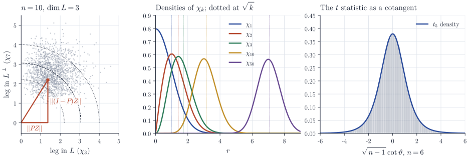
\[\sqrt{k - 1} \le \E R \le \sqrt k ,\]

so $R = \sqrt k + O_P(1)$: the length grows like $\sqrt k$ but fluctuates on a scale of order one. The middle panel of Figure 1 shows the densities $f_k$ moving to the right and keeping their width as $k$ grows.

The triangle

Theorem 1. Let $\R^n = L_1 \oplus \dots \oplus L_m$ be a decomposition into mutually orthogonal subspaces with $\dim L_j = d_j$, and write $P_j = P_{L_j}$. Then the vectors $P_1 Z, \dots, P_m Z$ are independent, and $\norm{P_j Z}^2 \sim \chi^2_{d_j}$ for each $j$.

Proof. Choose an orthonormal basis of $\R^n$ consisting of an orthonormal basis of $L_1$, followed by one of $L_2$, and so on, and let $Q = [Q_1 \ \cdots \ Q_m]$ be the orthogonal matrix with these basis vectors as columns, $Q_j$ holding the $d_j$ columns from $L_j$. The vector $Y = Q^\top Z$ is Gaussian with mean zero and covariance $Q^\top Q = I_n$, so its coordinates are independent standard normals. Partition $Y$ into blocks $Y_{(j)} = Q_j^\top Z$ of sizes $d_j$. Then $P_j = Q_jQ_j^\top$, so $P_jZ = Q_jY_{(j)}$ is a function of the block $Y_{(j)}$ alone, and the blocks are independent. Since $Q_j$ has orthonormal columns, $\norm{P_jZ} = \norm{Y_{(j)}}$, the length of a standard Gaussian vector in $\R^{d_j}$.

With $m = 2$, $L_1 = L$ of dimension $k$ and $L_2 = L^\perp$, the vectors $P_LZ$ and $(I - P_L)Z$ are orthogonal and sum to $Z$. They form a right triangle with independent legs of lengths $\chi_k$ and $\chi_{n-k}$ and hypotenuse $\chi_n$; Pythagoras’ theorem becomes the additivity $\chi^2_k + \chi^2_{n-k} = \chi^2_n$ for independent summands. The shape of the triangle is described by the angle $\theta \in [0, \pi/2]$ between $Z$ and $L$, and its size by $\norm{Z}$.

Proposition 2. For $0 < k < n$, $\cos^2\theta = \norm{P_LZ}^2/\norm{Z}^2$ has the $\mathrm{Beta}(k/2, (n-k)/2)$ distribution and is independent of $\norm{Z}$.

Proof. By Theorem 1, $A = \norm{P_LZ}^2$ and $B = \norm{(I-P_L)Z}^2$ are independent gamma variables with shapes $\alpha = k/2$, $\beta = (n-k)/2$ and common rate $1/2$. Their joint density is proportional to $a^{\alpha-1}b^{\beta-1}e^{-(a+b)/2}$. The map $(a, b) \mapsto (s, u) = (a + b, a/(a+b))$ is a bijection of $(0,\infty)^2$ onto $(0, \infty)\times(0,1)$ with inverse $a = su$, $b = s(1-u)$ and Jacobian determinant $s$, so $(S, U) = (A + B, A/(A+B))$ has density proportional to

\[(su)^{\alpha-1}\bigl(s(1-u)\bigr)^{\beta-1}e^{-s/2}\,s = u^{\alpha-1}(1-u)^{\beta-1}\cdot s^{\alpha+\beta-1}e^{-s/2} .\]

The density factorizes, so $U = \cos^2\theta$ is independent of $S = \norm{Z}^2$ and has the stated beta law.

The left panel of Figure 1 shows the pairs of legs for $n = 10$ and $k = 3$. The cloud is not rotationally symmetric, since the legs have different chi laws. Proposition 2 says that the distance from the origin is nevertheless independent of the polar angle: within every angular sector, the same proportion of points lies beyond each of the arcs drawn at quantiles of $\chi_{10}$.

Scatter of the two leg lengths of projections of a Gaussian vector with one highlighted right triangle, chi densities for several dimensions, and a histogram of the t statistic computed as a cotangent — Figure 1. Left: legs $(\Vert PZ\Vert, \Vert(I-P)Z\Vert)$ for 1,500 draws of $Z \sim N(0, I_{10})$ and a fixed three-dimensional subspace $L$, with one triangle highlighted; the arcs are the 10%, 50% and 90% quantiles of the hypotenuse $\Vert Z\Vert \sim \chi_{10}$. Middle: $\chi_k$ densities, concentrating near $\sqrt k$ with spread of order one. Right: $\sqrt{n-1}\cot\vartheta$ computed from the angle $\vartheta$ between the standardized data vector and the direction $\mathbf 1$, for $2 \times 10^5$ normal samples of size $n = 6$, against the $t_5$ density.

The sample mean, the sample variance and the t statistic

Let $X_1, \dots, X_n$ be independent $N(\mu, \sigma^2)$, put $Z = (X - \mu\mathbf 1)/\sigma \sim N(0, I_n)$, where $\mathbf 1 = (1, \dots, 1)^\top$, and take $L = \mathrm{span}(\mathbf 1)$, so $k = 1$. With the unit vector $e = \mathbf 1/\sqrt n$,

\[\begin{aligned} P_LZ &= \langle Z, e\rangle e, & \langle Z, e\rangle &= \frac{\sqrt n(\bar X - \mu)}{\sigma}, \\ (I - P_L)Z &= \frac{X - \bar X\mathbf 1}{\sigma}, & \norm{(I-P_L)Z}^2 &= \frac{(n-1)S^2}{\sigma^2}, \end{aligned}\]

where $S^2 = (n-1)^{-1}\sum_i(X_i - \bar X)^2$. Theorem 1 gives at once that $\bar X$ and $S^2$ are independent (they are functions of $P_LZ$ and $(I-P_L)Z$ respectively), that $(n-1)S^2/\sigma^2 \sim \chi^2_{n-1}$, and that $\sqrt n(\bar X - \mu)/\sigma \sim N(0,1)$.

Now measure the angle $\vartheta \in (0, \pi)$ between $Z$ and $e$ itself, so that $\langle Z, e\rangle = \norm{Z}\cos\vartheta$ and $\norm{(I-P_L)Z} = \norm{Z}\sin\vartheta$. The Student statistic is

\[T = \frac{\sqrt n(\bar X - \mu)}{S} = \frac{\langle Z, e\rangle}{\norm{(I-P_L)Z}/\sqrt{n-1}} = \sqrt{n-1}\,\cot\vartheta .\]

It is a function of the direction of the data vector alone, which is why it does not involve $\sigma$: rescaling the data changes the length of the triangle but not its shape. Its law is that of a standard normal divided by the square root of an independent $\chi^2_{n-1}/(n-1)$ variable, which is $t_{n-1}$. The t-test rejects $\mu = \mu_0$ when the vector $X - \mu_0\mathbf 1$ makes a small angle with the line spanned by $\mathbf 1$. The right panel of Figure 1 computes $T$ exactly this way, from angles, and recovers the $t_5$ density for $n = 6$.

The F test in linear models

Consider $Y = X\beta + \sigma\varepsilon$ with $\varepsilon \sim N(0, I_n)$ and a fixed design $X \in \R^{n\times p}$ of rank $p < n$. Let $L = \mathrm{col}(X)$, let $L_0 \subset L$ be the column space of a submodel, of dimension $p_0 < p$, and write $H$ and $H_0$ for the projections onto $L$ and $L_0$. The residual sums of squares of the two least squares fits are $\mathrm{RSS} = \norm{(I-H)Y}^2$ and $\mathrm{RSS}_0 = \norm{(I-H_0)Y}^2$.

Decompose $\R^n = L_0 \oplus (L \ominus L_0) \oplus L^\perp$, where $L \ominus L_0$ is the orthogonal complement of $L_0$ inside $L$, with dimensions $p_0$, $p - p_0$ and $n - p$; the corresponding projections are $H_0$, $H - H_0$ and $I - H$. Since $(I - H_0)Y = (H - H_0)Y + (I - H)Y$ is an orthogonal sum, $\mathrm{RSS}_0 - \mathrm{RSS} = \norm{(H - H_0)Y}^2$.

Proposition 3. If $X\beta \in L_0$, then

\[F = \frac{(\mathrm{RSS}_0 - \mathrm{RSS})/(p - p_0)}{\mathrm{RSS}/(n - p)} \sim F_{p - p_0,\, n - p},\]

the ratio of independent $\chi^2_{p-p_0}/(p-p_0)$ and $\chi^2_{n-p}/(n-p)$ variables.

Proof. Because $X\beta \in L_0 \subseteq L$, both $(I - H)$ and $(H - H_0)$ annihilate $X\beta$, so $(I-H)Y = \sigma(I-H)\varepsilon$ and $(H - H_0)Y = \sigma(H - H_0)\varepsilon$. Theorem 1 applied to $\varepsilon$ and the three-term decomposition shows that $\norm{(H-H_0)\varepsilon}^2 \sim \chi^2_{p-p_0}$ and $\norm{(I-H)\varepsilon}^2 \sim \chi^2_{n-p}$ are independent. The factor $\sigma^2$ cancels in the ratio.

Geometrically, $(I-H_0)Y$ is the hypotenuse of a right triangle with one leg in $L \ominus L_0$ and the other in $L^\perp$, and $F$ is $(n-p)/(p-p_0)$ times the squared cotangent of the angle between the hypotenuse and $L \ominus L_0$. Under the null hypothesis the residual of the small model points in a uniformly random direction within $L_0^\perp$, and a large $F$ means that it leans unusually far into the directions that the larger model can fit. For $p - p_0 = 1$, $F$ is the square of a t statistic for a single coefficient, mirroring the previous section. The same reasoning shows that $\hat\beta$, a function of $HY$, is independent of $\mathrm{RSS}$, which is what makes confidence regions for $\beta$ exact.

Remarks

Theorem 1 is a form of Cochran’s theorem, usually stated for quadratic forms $Z^\top A_jZ$ with symmetric $A_j$, $\sum_j A_j = I$ and $\sum_j\rank A_j = n$; the condition forces the $A_j$ to be projections onto mutually orthogonal subspaces, which reduces it to the version above. Under alternatives the projections acquire nonzero means, and the squared legs follow noncentral chi-squared laws whose noncentrality is the squared length of the projected mean (for the F test, $\norm{(H - H_0)X\beta}^2/\sigma^2$); this is how power calculations for the F test are done.

Treatments from this geometric point of view can be found in H. Scheffé, The Analysis of Variance, and G. A. F. Seber and A. J. Lee, Linear Regression Analysis.