A chi-square upper bound on the evidence, and the sandwich it makes with the ELBO
The evidence lower bound (ELBO) gives a computable lower bound on the log marginal likelihood \(\log p(y)\), and maximizing it over a variational family is equivalent to minimizing \(\mathrm{KL}(q\Vert \pi)\), where \(\pi\) is the posterior. An upper bound obtained in the same way would bracket \(\log p(y)\) and would come with its own variational problem. Dieng, Tran, Ranganath, Paisley and Blei (Variational inference via \(\chi\) upper bound minimization, NeurIPS 2017) proposed such a bound, the CUBO, and showed that minimizing it amounts to minimizing a \(\chi^2\) divergence from the posterior. Below, the bound and its basic properties are derived, and a one-dimensional example in which every quantity can be computed exactly shows what the \(\chi^2\) criterion does in practice.
Setting
Let \(z \in \R^d\) be latent, \(y\) the observed data, and \(p(y, z) = p(z)\, p(y \mid z)\) a joint density in \(z\) for the fixed observed \(y\). Assume the evidence \(p(y) = \int p(y, z) \, \dd z\) lies in \((0, \infty)\) and write \(\pi(z) = p(y, z)/p(y)\) for the posterior density. A variational density \(q\) is required to satisfy
\[q(z) > 0 \quad \text{whenever} \quad \pi(z) > 0, \tag{A}\]and with \(Z \sim q\) we define the importance weight \(W = p(y, Z)/q(Z)\). Under (A), \(\E_q W = \int_{\{q > 0\}} p(y, z) \, \dd z = p(y)\).
When \(\E_q \abs{\log W} < \infty\), the ELBO is \(\mathcal L(q) = \E_q \log W\), and writing \(\log W = \log p(y) + \log(\pi(Z)/q(Z))\) gives the familiar decomposition
\[\mathcal L(q) = \log p(y) - \mathrm{KL}(q\Vert\pi) \le \log p(y).\]The bound comes from Jensen’s inequality for the concave logarithm. Raising \(W\) to a power larger than one and taking the logarithm outside the expectation reverses the direction.
The bound
For \(n > 1\) define
\[\mathrm{CUBO}_n(q) = \frac1n \log \E_q\bigl[W^n\bigr] \in (-\infty, \infty],\]and recall the \(\chi^2\) divergence \(\chi^2(\pi\Vert q) = \int \pi^2/q \, \dd z - 1\), which is the \(f\)-divergence with \(f(t) = (t-1)^2\).
Proposition 1. Assume (A) and let \(n > 1\). Then
\[\mathrm{CUBO}_n(q) = \log p(y) + \frac1n \log \int \pi(z)^n q(z)^{1-n} \, \dd z \;\ge\; \log p(y),\]with equality if and only if \(q = \pi\) almost everywhere. In particular \(\mathrm{CUBO}_2(q) = \log p(y) + \tfrac12 \log\bigl(1 + \chi^2(\pi\Vert q)\bigr)\). Moreover \(n \mapsto \mathrm{CUBO}_n(q)\) is non-decreasing on \((1, \infty)\).
Proof. Since \(W = p(y)\, \pi(Z)/q(Z)\), we have \(\E_q W^n = p(y)^n \, \E_q[(\pi/q)^n(Z)] = p(y)^n \int_{\{q>0\}} \pi^n q^{1-n}\), and by (A) the integral may be taken over all of \(\R^d\). This is the displayed identity. The function \(t \mapsto t^n\) is strictly convex on \([0,\infty)\), so Jensen’s inequality and \(\E_q[\pi(Z)/q(Z)] = 1\) give \(\E_q[(\pi/q)^n] \ge 1\), with equality only if \(\pi/q\) is \(q\)-almost surely constant, hence equal to \(1\). For \(n = 2\) the integral is \(1 + \chi^2(\pi\Vert q)\). For monotonicity let \(1 < n < n'\); Jensen’s inequality for the convex map \(t \mapsto t^{n'/n}\) applied to \(W^n\) gives \((\E_q W^n)^{n'/n} \le \E_q W^{n'}\), and taking logarithms and dividing by \(n'\) gives \(\mathrm{CUBO}_n \le \mathrm{CUBO}_{n'}\).
The gap \(\tfrac1n \log \int \pi^n q^{1-n}\) equals \(\tfrac{n-1}{n} D_n(\pi\Vert q)\), where \(D_n\) is the Rényi divergence of order \(n\). So the CUBO is the upper half of a one-parameter family. Li and Turner (Rényi divergence variational inference, NeurIPS 2016) study \(\tfrac{1}{1-\alpha} \log \E_q W^{1-\alpha}\), which is the CUBO with \(n = 1 - \alpha\) when \(\alpha < 0\), is a lower bound for \(\alpha \in (0,1)\), and tends to the ELBO as \(\alpha \to 1\) under integrability conditions.
Together with the ELBO the bound gives a sandwich
\[\log p(y) - \mathrm{KL}(q\Vert \pi) \;=\; \mathcal L(q) \;\le\; \log p(y) \;\le\; \mathrm{CUBO}_2(q) \;=\; \log p(y) + \tfrac12 \log\bigl(1 + \chi^2(\pi\Vert q)\bigr),\]whose width \(\mathrm{CUBO}_2(q) - \mathcal L(q)\) involves divergences in both directions.
What the upper bound controls
The ELBO gap is a reverse divergence, which tolerates a \(q\) that misses parts of \(\pi\). The CUBO gap is of the forward type and penalizes the opposite failure: wherever \(\pi\) has mass and \(q\) is small, \(\pi^2/q\) is large. Two consequences make this precise.
Proposition 2. Assume (A).
- \(\tfrac12 \mathrm{KL}(\pi\Vert q) \le \mathrm{CUBO}_2(q) - \log p(y)\).
- Let \(Z_1, \dots, Z_S\) be independent draws from \(q\) and \(\hat p_S = S^{-1}\sum_{s=1}^S W_s\) the importance sampling estimate of the evidence. Then \(\E \hat p_S = p(y)\) and \(\Var(\hat p_S)/p(y)^2 = \chi^2(\pi\Vert q)/S\).
Proof. (1) By Jensen’s inequality for the concave logarithm under \(\pi\),
\[\mathrm{KL}(\pi\Vert q) = \E_\pi \log \frac{\pi(Z)}{q(Z)} \le \log \E_\pi \frac{\pi(Z)}{q(Z)} = \log \int \frac{\pi^2}{q} = \log\bigl(1 + \chi^2(\pi\Vert q)\bigr),\]and the right-hand side is \(2(\mathrm{CUBO}_2(q) - \log p(y))\) by Proposition 1. If \(\chi^2(\pi \Vert q) = \infty\) there is nothing to prove.
(2) Unbiasedness is \(\E_q W = p(y)\). The draws are independent, so \(\Var(\hat p_S) = \Var_q(W)/S\) and \(\Var_q(W) = \E_q W^2 - p(y)^2 = p(y)^2 \chi^2(\pi\Vert q)\) by Proposition 1.
By Proposition 1 the relative variance in part 2 can be written as
\[\frac{\Var(\hat p_S)}{p(y)^2} = \frac{\exp\bigl\{2\bigl(\mathrm{CUBO}_2(q) - \log p(y)\bigr)\bigr\} - 1}{S},\]which is the most useful reading of the bound. Within a family \(\mathcal Q\), the minimizer of \(\mathrm{CUBO}_2\) is the importance sampling proposal for the evidence with the smallest relative variance. This is why proposals for importance sampling are usually chosen with tails at least as heavy as those of the target: if \(q\) has lighter tails, \(\chi^2(\pi\Vert q)\) can be infinite.
A skew-normal posterior
Take a single latent \(z \in \R\) with prior \(\mathcal N(0,1)\) and one binary observation \(y = 1\) with \(\P(y = 1 \mid z) = \Phi(3z)\), where \(\Phi\) is the standard normal distribution function. If \(\varepsilon \sim \mathcal N(0,1)\) is independent of \(z\), then \(p(y{=}1) = \P(\varepsilon \le 3z) = \P(\varepsilon - 3z \le 0) = 1/2\) by symmetry, so \(\log p(y) = -\log 2\) exactly, and the posterior is the skew-normal density \(\pi(z) = 2\phi(z)\Phi(3z)\). Its left tail is much lighter than Gaussian, while for \(z \to +\infty\) the likelihood tends to one and \(\pi\) inherits the tail of the \(\mathcal N(0,1)\) prior. The variational family is \(\mathcal Q = \{\mathcal N(m, s^2)\}\).
This right tail determines which Gaussians have finite \(\chi^2\) divergence. For \(q = \mathcal N(m, s^2)\) and \(z \to +\infty\),
\[\frac{\pi(z)^2}{q(z)} \asymp \exp\Bigl\{ -\Bigl(1 - \frac{1}{2s^2}\Bigr) z^2 - \frac{m}{s^2} z \Bigr\},\]while for \(z \to -\infty\) the Mills-ratio bound \(\Phi(3z) \le \phi(3z)/(3\abs z)\) makes \(\pi(z)^2\) decay like \(e^{-10 z^2}\) up to polynomial factors, which is integrable against \(1/q\) whenever \(s^2 > 1/20\). Hence
\[\chi^2(\pi\Vert q) < \infty \iff s^2 > \tfrac12 \ \text{ or } \ \bigl(s^2 = \tfrac12 \text{ and } m > 0\bigr).\]The posterior has mean \(0.757\) and variance \(0.427\). Maximizing the ELBO gives \(q = \mathcal N(0.751, 0.351)\), with variance below that of the posterior as is usual for reverse-divergence fits; its \(\chi^2\) divergence is infinite, so \(\mathrm{CUBO}_2 = \infty\) and importance weights drawn from it have infinite variance, although the density plot shows nothing alarming. Minimizing \(\mathrm{CUBO}_2\) gives \(q = \mathcal N(0.744, 0.505)\), wider than the posterior and pressed against the constraint \(s^2 > 1/2\). At these optima \(\mathcal L = -0.737\) and \(\mathrm{CUBO}_2 = -0.654\), bracketing \(\log p(y) = -0.693\).
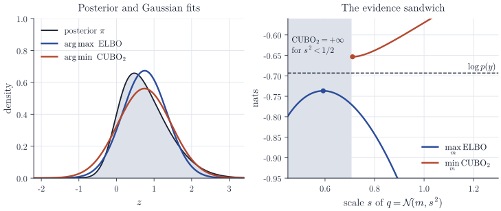
The constraint in this example is a general feature. If the likelihood stays bounded away from zero along some direction, the posterior tail in that direction is the prior tail. In one dimension, if \(\pi(z) \ge c\, \phi(z/\tau)/\tau\) for all large \(z\), the computation above shows that a Gaussian \(q\) has finite \(\chi^2(\pi\Vert q)\) only if \(s^2 \ge \tau^2/2\), however concentrated the bulk of the posterior is. Minimizing the \(\chi^2\) divergence over a Gaussian family can therefore produce an approximation much wider than the posterior, which is appropriate for importance sampling and less so as a summary of posterior uncertainty.
Estimating and optimizing the bound
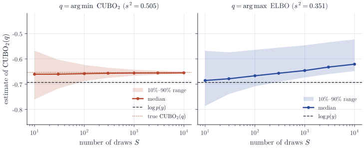
The ELBO is an expectation and has unbiased Monte Carlo estimates. The CUBO is a logarithm of an expectation, and the natural estimate \(\widehat{\mathrm{CUBO}}_{2,S} = \tfrac12 \log\bigl(S^{-1} \sum_s W_s^2\bigr)\) is biased downward: Jensen’s inequality gives \(\E\, \widehat{\mathrm{CUBO}}_{2,S} \le \mathrm{CUBO}_2(q)\). A finite-sample estimate is therefore not guaranteed to lie above \(\log p(y)\). The precision of the estimate depends on the fourth moment of \(W\), and by the same tail computation \(\E_q W^4 = \infty\) for every Gaussian \(q\) with \(s^2 < 3/4\) in the example. At the CUBO-optimal \(q\) the estimate of \(\E_q W^2\) thus has infinite variance, even though its mean is finite.
Figure 2 shows both effects. At the CUBO-optimal \(q\) the estimates converge to the true value, but for small \(S\) a sizeable fraction falls below \(\log p(y)\). At the ELBO-optimal \(q\), where \(\E_q W^2 = \infty\), the strong law of large numbers for non-negative variables gives \(\widehat{\mathrm{CUBO}}_{2,S} \to \infty\) almost surely; every individual estimate is finite and the drift upward is slow, so the divergence is easy to miss in practice.
For optimization, the logarithm can be dropped: since \(t \mapsto \tfrac1n \log t\) is increasing, minimizing \(\mathrm{CUBO}_n\) over \(\mathcal Q\) is the same as minimizing \(\E_q W^n\), which is the objective Dieng et al. work with; unlike the CUBO itself, it admits unbiased Monte Carlo gradient estimates. With a reparametrization \(Z = g_\lambda(\varepsilon)\), \(\varepsilon \sim r\), and \(W_\lambda(\varepsilon) = p(y, g_\lambda(\varepsilon))/q_\lambda(g_\lambda(\varepsilon))\),
\[\nabla_\lambda \E_{q_\lambda} W^n = \E_r\bigl[ n\, W_\lambda(\varepsilon)^{n-1} \nabla_\lambda W_\lambda(\varepsilon) \bigr],\]provided differentiation under the integral is justified, for instance by a \(\lambda\)-uniform integrable bound on \(\abs{\nabla_\lambda W_\lambda^n}\) near the current parameter. The bound is not automatic. The integrand equals \(n W_\lambda^n \nabla_\lambda \log W_\lambda\), so the second moment of the gradient estimator is \(n^2\E_r\bigl[W_\lambda^{2n} \norm{\nabla_\lambda \log W_\lambda}^2\bigr]\). In the example with \(n = 2\) and \(\lambda = (m, \log s)\), the factor \(\norm{\nabla_\lambda \log W_\lambda}^2\) grows like \(z^2\) in the right tail, and the second moment is infinite for every Gaussian with \(s^2 < 3/4\). In practice \(W\) is also computed on the log scale and rescaled by a running constant to avoid overflow, which changes the objective only by a positive factor.
Remarks
The upper bound complements the ELBO on two counts. It yields mass-covering approximations, controlling \(\mathrm{KL}(\pi\Vert q)\) through Proposition 2, and it is the natural objective when \(q\) will be used as an importance sampling proposal. Its weaknesses are the other side of the same coin: it is infinite whenever \(q\) has lighter tails than \(\pi^2\) requires, its Monte Carlo estimates are biased downward, and its gradients are heavy-tailed. The sandwich \(\mathcal L(q) \le \log p(y) \le \mathrm{CUBO}_2(q)\) is exact for exact expectations, but a bracket built from finite-sample estimates is only approximate on the upper side.