Conjugate gradients: conjugate directions, Krylov subspaces and the square-root speed-up
Steepest descent on an elongated quadratic bowl wastes most of its effort: each step undoes part of the progress of the previous ones, and the iterates zig-zag across the valley. Conjugate gradients fixes this with a different choice of search directions, chosen so that minimizing along a new direction never spoils the minimization already done along the old ones. The resulting method costs the same per iteration as steepest descent, a single product with the matrix, and it converges in a number of iterations governed by the square root of the condition number.
Setting
Let \(A \in \R^{n \times n}\) be symmetric positive definite, \(b \in \R^n\), and
\[f(x) = \tfrac12 x^\top A x - b^\top x .\]The unique minimizer is \(x_\star = A^{-1}b\), the gradient is \(\nabla f(x) = Ax - b = -r(x)\) with \(r(x) = b - Ax\) the residual, and completing the square gives
\[f(x) - f(x_\star) = \tfrac12 (x - x_\star)^\top A (x - x_\star) = \tfrac12 \lVert x - x_\star\rVert_A^2 .\]Minimizing \(f\) and solving \(Ax = b\) are the same problem, and the natural error measure is the energy norm \(\lVert\cdot\rVert_A\). Write \(\kappa = \lambda_{\max}(A)/\lambda_{\min}(A)\) for the condition number. For reference, steepest descent with exact line searches satisfies \(\lVert x_{k} - x_\star\rVert_A \le \bigl(\tfrac{\kappa-1}{\kappa+1}\bigr)^k \lVert x_0 - x_\star\rVert_A\), a consequence of the Kantorovich inequality, and the bound is attained for suitable starting points (Nocedal and Wright, Numerical Optimization). With \(\kappa = 1000\) that is a reduction of about \(0.2\%\) per step.
Conjugate directions
Nonzero vectors \(p_0, \dots, p_{k-1}\) are conjugate (with respect to \(A\)) if \(p_i^\top A p_j = 0\) for \(i \neq j\). Conjugate vectors are linearly independent, since applying \(p_j^\top A\) to a vanishing linear combination isolates the \(j\)th coefficient. The point of conjugacy is that it decouples the line searches.
Lemma 1 (expanding subspaces). Let \(p_0, \dots, p_{k-1}\) be conjugate, and define \(x_{j+1} = x_j + \alpha_j p_j\) with the exact line-search step \(\alpha_j = p_j^\top r_j / p_j^\top A p_j\), where \(r_j = b - Ax_j\). Then \(x_k\) minimizes \(f\) over the affine set \(x_0 + \mathrm{span}\{p_0, \dots, p_{k-1}\}\), and \(r_k\) is orthogonal to \(p_0, \dots, p_{k-1}\).
Proof. For \(x = x_0 + \sum_{i<k} \gamma_i p_i\), conjugacy kills the cross terms in the quadratic part:
\[f(x) = f(x_0) + \sum_{i<k} \Bigl( \tfrac12 \gamma_i^2\, p_i^\top A p_i - \gamma_i\, p_i^\top r_0 \Bigr).\]Each summand depends on one \(\gamma_i\) only and is minimized at \(\gamma_i = p_i^\top r_0 / p_i^\top A p_i\). The sequential steps produce these values: \(r_i = r_0 - \sum_{j<i}\alpha_j A p_j\), so \(p_i^\top r_i = p_i^\top r_0\) by conjugacy, and \(\alpha_i = \gamma_i\). At the minimizer over the affine set the gradient \(-r_k\) is orthogonal to the set’s direction space.
With \(n\) conjugate directions the span is all of \(\R^n\), so \(x_n = x_\star\) in exact arithmetic, whatever the conditioning. Conjugate directions exist, for instance the eigenvectors of \(A\), but computing those is harder than solving the system. Conjugate gradients generates them on the fly.
The algorithm
Start from \(x_0\), set \(r_0 = b - Ax_0\) and \(p_0 = r_0\), and for \(k = 0, 1, \dots\) while \(r_k \neq 0\),
\[\begin{aligned} \alpha_k &= \frac{r_k^\top r_k}{p_k^\top A p_k}, & x_{k+1} &= x_k + \alpha_k p_k, & r_{k+1} &= r_k - \alpha_k A p_k, \\[6pt] \beta_k &= \frac{r_{k+1}^\top r_{k+1}}{r_k^\top r_k}, & p_{k+1} &= r_{k+1} + \beta_k p_k . & & \end{aligned}\]Each iteration needs one product \(Ap_k\), a few inner products and a few vector updates, and storage for four vectors. The new direction is the new residual, which is the steepest descent direction, corrected by a multiple of the previous direction. Write \(\mathcal K_k = \mathrm{span}\{r_0, Ar_0, \dots, A^{k-1}r_0\}\) for the Krylov subspaces.
Theorem 2. Suppose \(r_0, \dots, r_k\) are nonzero. Then the residuals \(r_0, \dots, r_k\) are mutually orthogonal, the directions \(p_0, \dots, p_k\) are conjugate, and
\[\mathrm{span}\{r_0, \dots, r_k\} = \mathrm{span}\{p_0, \dots, p_k\} = \mathcal K_{k+1}.\]Moreover \(\alpha_k\) is the exact line-search step \(p_k^\top r_k/p_k^\top A p_k\).
Proof. Induction on \(k\); the case \(k = 0\) is trivial. Assume the claims up to \(k\), and that \(r_{k+1} \neq 0\).
Line search. By Lemma 1 applied with the conjugate \(p_0, \dots, p_{k-1}\), \(r_k \perp p_{k-1}\), so \(p_k^\top r_k = r_k^\top r_k + \beta_{k-1}p_{k-1}^\top r_k = r_k^\top r_k\), and \(\alpha_k\) is the exact step.
Spans. \(p_k \in \mathcal K_{k+1}\) gives \(Ap_k \in \mathcal K_{k+2}\), hence \(r_{k+1} = r_k - \alpha_k Ap_k \in \mathcal K_{k+2}\) and \(p_{k+1} = r_{k+1} + \beta_k p_k \in \mathcal K_{k+2}\). Once orthogonality is shown, the \(k+2\) nonzero residuals are linearly independent, so their span, which lies in \(\mathcal K_{k+2}\) of dimension at most \(k+2\), equals it; the same holds for the directions, which are conjugate and hence independent. (They are nonzero: \(r_{k+1} \perp p_k\) by Lemma 1, so \(\lVert p_{k+1}\rVert \ge \lVert r_{k+1}\rVert > 0\).)
Orthogonality. The steps so far are exact line searches along conjugate directions, so by Lemma 1 \(r_{k+1} \perp \mathrm{span}\{p_0, \dots, p_k\} = \mathrm{span}\{r_0, \dots, r_k\}\).
Conjugacy. For \(j < k\), \(p_{k+1}^\top A p_j = r_{k+1}^\top Ap_j + \beta_k p_k^\top A p_j = r_{k+1}^\top A p_j = 0\), because \(Ap_j \in \mathcal K_{j+2} \subseteq \mathrm{span}\{p_0, \dots, p_k\}\), which is orthogonal to \(r_{k+1}\). For \(j = k\), substitute \(Ap_k = (r_k - r_{k+1})/\alpha_k\) and \(p_k^\top A p_k = r_k^\top r_k/\alpha_k\):
\[p_{k+1}^\top A p_k = \frac{-r_{k+1}^\top r_{k+1} + \beta_k\, r_k^\top r_k}{\alpha_k} = 0\]by the choice of \(\beta_k\).
Krylov optimality and its consequences
Combining Lemma 1 with Theorem 2, \(x_k\) minimizes \(f\), equivalently \(\lVert x - x_\star\rVert_A\), over \(x_0 + \mathcal K_k\). Every point of that set has the form \(x_0 + q(A)r_0\) for a polynomial \(q\) of degree less than \(k\), and since \(r_0 = A(x_\star - x_0)\) its error is
\[x_0 + q(A)r_0 - x_\star = \bigl(I - Aq(A)\bigr)(x_0 - x_\star) = P(A)(x_0 - x_\star),\]where \(P(\lambda) = 1 - \lambda q(\lambda)\) ranges over the set \(\mathcal P_k\) of polynomials of degree at most \(k\) with \(P(0) = 1\).
Theorem 3. Let \(\lambda_1, \dots, \lambda_n\) be the eigenvalues of \(A\). The conjugate gradient iterates satisfy
\[\lVert x_k - x_\star\rVert_A = \min_{P \in \mathcal P_k} \lVert P(A)(x_0 - x_\star)\rVert_A \le \min_{P \in \mathcal P_k} \max_{i} \lvert P(\lambda_i)\rvert \; \lVert x_0 - x_\star\rVert_A .\]Proof. The equality is the optimality just described. For the inequality, expand \(x_0 - x_\star = \sum_i c_i v_i\) in orthonormal eigenvectors of \(A\). Then \(\lVert P(A)(x_0 - x_\star)\rVert_A^2 = \sum_i \lambda_i P(\lambda_i)^2 c_i^2 \le \max_i P(\lambda_i)^2 \sum_i \lambda_i c_i^2\), and the last sum is \(\lVert x_0 - x_\star\rVert_A^2\).
Conjugate gradients is therefore as good as the best polynomial on the spectrum, chosen adaptively and without knowledge of the eigenvalues. Three consequences follow by choosing particular polynomials.
Finite termination by distinct eigenvalues. If \(A\) has only \(m\) distinct eigenvalues \(\mu_1, \dots, \mu_m\), the polynomial \(\prod_{l}(1 - \lambda/\mu_l)\) lies in \(\mathcal P_m\) and vanishes on the spectrum, so \(x_m = x_\star\).
The square-root rate. Let \(T_k\) be the Chebyshev polynomial of degree \(k\), which satisfies \(\lvert T_k\rvert \le 1\) on \([-1, 1]\) and \(T_k(z) = \tfrac12\bigl[(z + \sqrt{z^2-1})^k + (z - \sqrt{z^2-1})^k\bigr] \ge \tfrac12 (z + \sqrt{z^2-1})^k\) for \(z \ge 1\). The polynomial
\[P(\lambda) = \frac{T_k\bigl((\lambda_{\max} + \lambda_{\min} - 2\lambda)/(\lambda_{\max} - \lambda_{\min})\bigr)}{T_k(z_0)}, \qquad z_0 = \frac{\lambda_{\max} + \lambda_{\min}}{\lambda_{\max} - \lambda_{\min}} = \frac{\kappa + 1}{\kappa - 1},\]belongs to \(\mathcal P_k\) and is bounded by \(1/T_k(z_0)\) on \([\lambda_{\min}, \lambda_{\max}]\), which contains the spectrum. Since \(z_0 + \sqrt{z_0^2 - 1} = (\kappa + 1 + 2\sqrt\kappa)/(\kappa - 1) = (\sqrt\kappa + 1)/(\sqrt\kappa - 1)\),
\[\lVert x_k - x_\star\rVert_A \le 2\Bigl(\frac{\sqrt\kappa - 1}{\sqrt\kappa + 1}\Bigr)^{k} \lVert x_0 - x_\star\rVert_A .\]For large \(\kappa\) the factor per step is about \(1 - 2/\sqrt\kappa\) against \(1 - 2/\kappa\) for steepest descent, so reducing the error by a fixed factor takes \(O(\sqrt\kappa)\) iterations instead of \(O(\kappa)\).
Clusters and outliers. The Chebyshev bound uses only the extreme eigenvalues and is pessimistic when the spectrum is clustered. Suppose all eigenvalues lie in \([1, 2]\) except \(m\) outliers \(\mu_1, \dots, \mu_m > 2\). Multiply the Chebyshev polynomial for \([1, 2]\) by \(\prod_l (1 - \lambda/\mu_l)\): the product kills the outliers, and on \([1, 2]\) each factor \(1 - \lambda/\mu_l\) lies in \((0, 1)\). Hence
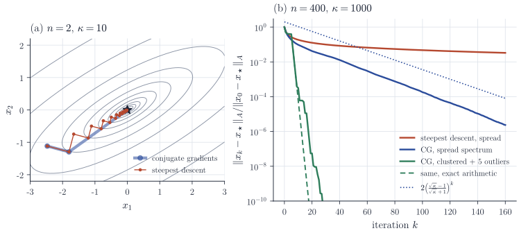
\[\lVert x_{m+j} - x_\star\rVert_A \le 2\Bigl(\frac{\sqrt2 - 1}{\sqrt2 + 1}\Bigr)^{j} \lVert x_0 - x_\star\rVert_A ,\]so in exact arithmetic each outlier costs at most one extra iteration and the rest proceeds at the rate of the cluster, a factor of about \(0.17\) per step here, regardless of how large the outliers are. In floating point the picture is less clean, as Figure 1(b) shows and the last section explains.
Practice
The clustering analysis is the rationale for preconditioning. Solving \(M^{-1}Ax = M^{-1}b\) with a symmetric positive definite \(M\) that is cheap to invert and approximates \(A\) amounts to running conjugate gradients in the inner product defined by \(M\), with an iteration matrix similar to \(M^{-1/2}AM^{-1/2}\). A good preconditioner clusters the spectrum of this matrix near one, leaving a few outliers.
In floating point, the residuals gradually lose orthogonality and finite termination is lost. The method still converges, and the Chebyshev bound, which depends only on the extreme eigenvalues, remains a reliable guide. The bounds that exploit the fine structure of the spectrum are more fragile: once an outlying eigenvalue has been resolved, rounding errors let it reappear in later iterations, and each reappearance costs extra steps. This is the delay seen in Figure 1(b), and it is most pronounced for large, well-separated outliers. Greenbaum, Iterative Methods for Solving Linear Systems, analyses this behaviour; roughly, finite-precision conjugate gradients behaves like exact conjugate gradients applied to a larger matrix whose eigenvalues lie in small intervals around those of \(A\). In statistics the method is useful whenever \(A\) is available only through products: penalized least-squares systems \((X^\top X + \lambda I)\beta = X^\top y\), where each product costs two passes over the data; Gaussian process regression, where \((K + \sigma^2 I)\alpha = y\) must be solved for a large kernel matrix; and truncated Newton methods, in which conjugate gradients solves the Newton system approximately using Hessian–vector products. For general nonlinear objectives, the same recursion with \(\beta_k\) computed from gradients gives the nonlinear conjugate gradient methods, which need restarts and inexact line searches but inherit the behaviour described here near a minimum with positive definite Hessian.