Control variates: a regression adjustment inside a Monte Carlo average
The plain Monte Carlo estimator of \(\theta = \E f(X)\) from independent draws \(X_1, \dots, X_n\) has standard error \(\sigma_f/\sqrt n\), where \(\sigma_f^2 = \Var f(X)\). The rate \(n^{-1/2}\) cannot be improved by averaging more cleverly, but the constant can. Control variates reduce \(\sigma_f\) by subtracting from \(f(X)\) a quantity whose expectation is known exactly and whose fluctuations track those of \(f(X)\). The resulting estimator is a regression estimator, and much of what is known about it is ordinary least squares in disguise.
One control
Let \(g(X)\) be a real random variable with known mean \(\mu_g\) and \(0 < \sigma_g^2 = \Var g(X) < \infty\), and assume \(\sigma_f^2 < \infty\). For any fixed \(\beta \in \R\),
\[\hat\theta_\beta = \frac1n \sum_{i=1}^n \bigl\{ f(X_i) - \beta\bigl(g(X_i) - \mu_g\bigr) \bigr\}\]is unbiased for \(\theta\), with variance \(n^{-1}(\sigma_f^2 - 2\beta\sigma_{fg} + \beta^2 \sigma_g^2)\), where \(\sigma_{fg} = \Cov(f(X), g(X))\). The quadratic in \(\beta\) is minimized at
\[\beta^* = \frac{\sigma_{fg}}{\sigma_g^2}, \qquad \Var \hat\theta_{\beta^*} = \frac{\sigma_f^2 (1 - \rho^2)}{n}, \qquad \rho = \Corr\bigl(f(X), g(X)\bigr).\]A correlation of \(0.95\) reduces the variance by a factor of about ten, and \(0.995\) by a factor of a hundred. The sign of \(\rho\) does not matter, and every \(\beta\) strictly between \(0\) and \(2\beta^*\) reduces the variance.
The coefficient \(\beta^*\) is the slope of the population least-squares line of \(f(X)\) on \(g(X)\), and \(f(X) - \beta^*(g(X) - \mu_g)\) is the intercept plus the regression residual. Subtracting the control removes the part of \(f\) explained linearly by \(g\), and what remains has variance \(\sigma_f^2(1 - \rho^2)\).
Several controls
With a vector of controls \(g(X) \in \R^k\) with known mean \(\mu_g\) and nonsingular covariance \(\Sigma_{gg}\), and \(\Sigma_{gf} = \Cov(g(X), f(X)) \in \R^k\), the same computation gives
\[\begin{aligned} \Var\bigl(f(X) - \beta^\top (g(X) - \mu_g)\bigr) &= \sigma_f^2 - 2\beta^\top \Sigma_{gf} + \beta^\top \Sigma_{gg} \beta \\ &= \sigma_f^2 - \Sigma_{gf}^\top \Sigma_{gg}^{-1} \Sigma_{gf} + (\beta - \beta^*)^\top \Sigma_{gg} (\beta - \beta^*), \end{aligned}\]with \(\beta^* = \Sigma_{gg}^{-1}\Sigma_{gf}\). The minimum is \(\sigma_{\mathrm{res}}^2 = \sigma_f^2(1 - R^2)\), where \(R^2 = \Sigma_{gf}^\top \Sigma_{gg}^{-1} \Sigma_{gf} / \sigma_f^2\) is the squared multiple correlation of \(f(X)\) with \(g(X)\). Geometrically, \(\sigma_{\mathrm{res}}^2\) is the squared \(L^2\) distance from \(f(X)\) to the affine span of \(1, g_1(X), \dots, g_k(X)\). Adding controls can only decrease it.
Estimating the coefficient
The optimal coefficient involves the unknown \(\Sigma_{gf}\), so in practice it is estimated from the same draws. Let \(\hat\beta\) be the least-squares slope in the regression of \(f(X_i)\) on \(g(X_i)\) with an intercept, and define \(\hat\theta_{\mathrm{cv}} = \hat\theta_{\hat\beta}\). Since the least-squares fit passes through the point of means \((\bar g, \bar f)\), we can write
\[\hat\theta_{\mathrm{cv}} = \bar f - \hat\beta^\top (\bar g - \mu_g) = \hat a + \hat\beta^\top \mu_g ,\]where \(\hat a\) is the fitted intercept. In words, \(\hat\theta_{\mathrm{cv}}\) is the fitted regression function evaluated at the known mean of the controls, while the plain average \(\bar f\) is the same function evaluated at their sample mean. If the controls are centred, so that \(\mu_g = 0\), the estimator is the intercept.
Proposition 1. Assume \(\E f(X)^2 < \infty\), \(\E \norm{g(X)}^2 < \infty\) and \(\Sigma_{gg}\) nonsingular. Then \(\hat\theta_{\mathrm{cv}} \to \theta\) almost surely and
\[\sqrt n\,\bigl(\hat\theta_{\mathrm{cv}} - \theta\bigr) \xrightarrow{d} N\bigl(0, \sigma_{\mathrm{res}}^2\bigr), \qquad n \to \infty .\]The residual mean square of the regression is a consistent estimator of \(\sigma_{\mathrm{res}}^2\).
Proof. The sample covariances converge almost surely to their population values by the strong law of large numbers; the cross moments are integrable by the Cauchy–Schwarz inequality. Since \(\Sigma_{gg}\) is nonsingular, the sample covariance matrix of the controls is nonsingular for all large \(n\) almost surely, and \(\hat\beta \to \beta^*\) almost surely by continuity of matrix inversion. Now
\[\hat\theta_{\mathrm{cv}} - \hat\theta_{\beta^*} = -(\hat\beta - \beta^*)^\top (\bar g - \mu_g).\]The estimator \(\hat\theta_{\beta^*}\) is an average of independent copies of \(f(X) - \beta^{*\top}(g(X) - \mu_g)\), which has mean \(\theta\) and variance \(\sigma_{\mathrm{res}}^2\), so the central limit theorem gives \(\sqrt n(\hat\theta_{\beta^*} - \theta) \xrightarrow{d} N(0, \sigma_{\mathrm{res}}^2)\). The difference above, multiplied by \(\sqrt n\), is the product of \(\hat\beta - \beta^* \to 0\) almost surely and \(\sqrt n(\bar g - \mu_g)\), which converges in distribution and is therefore bounded in probability. It tends to zero in probability, and Slutsky’s lemma gives the limit. Almost sure convergence follows from the same decomposition and the strong law. The residual mean square is a continuous function of the sample moments and converges to \(\sigma_f^2 - \Sigma_{gf}^\top\Sigma_{gg}^{-1}\Sigma_{gf}\).
Two finite-sample effects are hidden in the first-order statement. The estimator is biased, because \(\hat\beta\) and \(\bar g\) are dependent; the bias is \(-\E[(\hat\beta - \beta^*)^\top(\bar g - \mu_g)]\), which under moment conditions is of order \(1/n\), negligible beside the \(n^{-1/2}\) standard error. If exact unbiasedness matters, \(\beta\) can be estimated from a separate pilot sample, which makes it independent of the draws used in the average. Second, estimating \(k\) coefficients inflates the variance for small \(n\); with \(k\) fixed the inflation disappears as \(n\) grows, but \(k\) should stay small relative to \(n\).
An example
Let \(Z \sim N(\mu, \sigma^2)\) with \(\mu = 0.5\), \(\sigma = 1.5\), and let \(f(z) = \log(1 + e^{z})\), the softplus function, which appears in the log-likelihood of logistic regression. The integral \(\theta = \E f(Z)\) has no closed form; quadrature gives \(\theta = 1.197\) and \(\sigma_f^2 = 0.854\).
Controls come from cruder approximations of \(f\) whose expectations are known. A second-order Taylor expansion around \(\mu\) is
\[f(z) \approx f(\mu) + s(\mu)(z - \mu) + \tfrac12 s(\mu)\bigl(1 - s(\mu)\bigr)(z - \mu)^2, \qquad s(t) = \frac{1}{1 + e^{-t}},\]which suggests the centred controls \(g_1 = Z - \mu\) and \(g_2 = (Z - \mu)^2 - \sigma^2\), both of mean zero. Computing the moments by quadrature, \(g_1\) alone gives \(R^2 = 0.910\), a variance reduction by a factor of \(11\), and the pair gives \(R^2 = 0.9976\), a factor of about \(420\). The optimal coefficients \((0.588, 0.086)\) differ from the Taylor coefficients \((0.622, 0.118)\), because least squares fits \(f\) over the whole distribution of \(Z\), not only near \(\mu\); plugging in the Taylor coefficients instead still reduces the variance, by a factor of about \(58\).
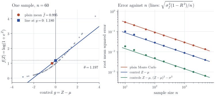
The left panel of Figure 1 shows the mechanism on one sample. The draws happen to have \(\bar g < 0\), so the plain mean underestimates \(\theta\); the regression line converts the known shortfall of the control into a correction of the estimate, moving it from \(0.995\) to \(1.180\). The right panel confirms Proposition 1: the three error curves are parallel lines of slope \(-1/2\) on the log–log scale, separated by the factors \(\sqrt{11}\) and \(\sqrt{420}\), and the finite-sample inflation from estimating two coefficients is confined to the smallest sample sizes.
Where controls come from
The example used a Taylor expansion, and this is typical: any tractable approximation \(\tilde f\) with known expectation gives a control \(\tilde f(X) - \E\tilde f(X)\), and the regression coefficient corrects for the quality of the approximation automatically. Other common sources are the same simulation run under a simpler model (in option pricing, a geometric average as a control for an arithmetic one), and quantities whose mean is known by symmetry.
A systematic source is Stein’s identity. If \(Z \sim N(\mu, \sigma^2)\) and \(h\) is absolutely continuous with \(\E\abs{h'(Z)} < \infty\), then \(\E[(Z - \mu) h(Z)] = \sigma^2 \E h'(Z)\), so \((Z - \mu)h(Z) - \sigma^2 h'(Z)\) has mean zero for every such \(h\). The choices \(h = 1\) and \(h(z) = z - \mu\) give exactly \(g_1\) and \(g_2\). For a general density \(p\) the analogous mean-zero functions are \(h'(X) + h(X)\,(\log p)'(X)\), valid when the boundary terms vanish in the integration by parts. This works when \(p\) is known only up to its normalizing constant, so it applies to MCMC output, and it underlies the zero-variance control variates of Mira, Solgi and Imparato (Statistics and Computing, 2013) and the control functionals of Oates, Girolami and Chopin (Journal of the Royal Statistical Society, Series B, 2017).
Remarks
With correlated draws, as in MCMC, the coefficient that minimizes the asymptotic variance involves the autocovariances of \(f\) and \(g\), and the least-squares coefficient is no longer optimal in general, although it remains a consistent and often effective choice. The same estimator appears in survey sampling as the regression estimator, with known population means of auxiliary variables playing the role of \(\mu_g\). Glasserman’s Monte Carlo Methods in Financial Engineering treats control variates alongside the other standard variance reduction methods.