Square roots of a covariance matrix: Cholesky, eigen and symmetric factors of the multivariate normal

The usual recipe for simulating $X \sim N_p(\mu, \Sigma)$ is to factor $\Sigma = AA^\top$, draw independent standard normals $Z$ and return $\mu + AZ$. Several factorizations do the job, most often the Cholesky factorization and the eigendecomposition. They produce the same distribution but different random vectors, and each choice exposes a different aspect of the structure of $\Sigma$. Below we identify which factors are allowed, how they are related to each other and to the singular value decomposition, and what each one means probabilistically.

Any factor gives the same law

A random vector $X$ in $\R^p$ is multivariate normal with mean $\mu$ and covariance $\Sigma$ if its characteristic function is $\E e^{\mathrm i t^\top X} = \exp(\mathrm i t^\top \mu - \tfrac12 t^\top \Sigma t)$ for all $t \in \R^p$. Here $\Sigma$ is symmetric positive semi-definite, possibly singular.

Proposition 1. Let $Z \sim N_k(0, I_k)$ and $A \in \R^{p \times k}$. Then $\mu + AZ \sim N_p(\mu, AA^\top)$. Conversely, for every positive semi-definite $\Sigma$ and every $k \ge \rank \Sigma$ there is $A \in \R^{p \times k}$ with $AA^\top = \Sigma$.

Proof. Independence of the coordinates of $Z$ gives $\E e^{\mathrm i s^\top Z} = e^{-\lVert s\rVert^2/2}$ for $s \in \R^k$. With $s = A^\top t$,

\[\E e^{\mathrm i t^\top(\mu + AZ)} = e^{\mathrm i t^\top\mu}\, e^{-\lVert A^\top t\rVert^2/2} = \exp\bigl(\mathrm i t^\top\mu - \tfrac12 t^\top AA^\top t\bigr).\]

For the converse, write $\Sigma = \sum_{j=1}^r \lambda_j u_j u_j^\top$ with $r = \rank\Sigma$, orthonormal $u_j$ and $\lambda_j > 0$, and take the columns of $A$ to be $\sqrt{\lambda_j}\, u_j$ for $j \le r$, followed by $k - r$ zero columns.

So the law of $\mu + AZ$ depends on $A$ only through $AA^\top$. The next result identifies exactly how much freedom is left.

Proposition 2. Let $A, B \in \R^{p \times k}$. Then $AA^\top = BB^\top$ if and only if $B = AQ$ for some orthogonal $Q \in \R^{k \times k}$.

Proof. If $B = AQ$ then $BB^\top = AQQ^\top A^\top = AA^\top$. Conversely, $AA^\top = BB^\top$ means $\lVert A^\top x\rVert^2 = \lVert B^\top x\rVert^2$ for every $x \in \R^p$. Hence the map $A^\top x \mapsto B^\top x$ is well defined on the column space $\mathcal R(A^\top)$ (if $A^\top x = A^\top x'$ then $\lVert B^\top(x - x')\rVert = 0$), linear, and norm preserving, so it is an isometry of $\mathcal R(A^\top)$ onto $\mathcal R(B^\top)$. Both subspaces of $\R^k$ have dimension $\rank(AA^\top)$, so their orthogonal complements have equal dimension, and any isometry between the complements extends the map to an orthogonal $Q_0$ on $\R^k$ with $Q_0 A^\top = B^\top$. Take $Q = Q_0^\top$.

Proposition 2 is the rotational invariance of $N_k(0, I_k)$ seen from the other side: $QZ$ has the same law as $Z$, so $AQZ$ and $AZ$ have the same law.

The SVD of a factor

Take any factor $A \in \R^{p \times k}$ of $\Sigma$ and write its singular value decomposition $A = UDV^\top$, with $U \in \R^{p \times p}$ and $V \in \R^{k \times k}$ orthogonal and $D$ rectangular diagonal. Then

\[\Sigma = AA^\top = U (DD^\top) U^\top\]

is an eigendecomposition of $\Sigma$. The left singular vectors and singular values of every factor are the eigenvectors of $\Sigma$ and the square roots of its eigenvalues; the right singular vectors $V$ carry exactly the orthogonal freedom of Proposition 2. Different factors are different choices of $V$.

This has a sample counterpart that matters numerically. If $x_1, \dots, x_n \in \R^p$ are observations with mean $\bar x$ and $X_c$ is the centred $n \times p$ data matrix, the sample covariance is $S = n^{-1} X_c^\top X_c$, so $n^{-1/2} X_c^\top$ is a $p \times n$ factor of $S$. The principal axes and variances of the sample are therefore the right singular vectors and squared singular values (divided by $n$) of $X_c$, and they can be computed from the SVD of the data without forming $S$, which avoids squaring the condition number.

Three factors and what they mean

Assume $\Sigma \succ 0$ for the moment and write $\Sigma = U\Lambda U^\top$ with $\Lambda = \diag(\lambda_1, \dots, \lambda_p)$, $\lambda_1 \ge \cdots \ge \lambda_p > 0$. Three factors are in common use:

the eigen factor $U\Lambda^{1/2}$;
the symmetric square root $\Sigma^{1/2} = U\Lambda^{1/2}U^\top$, the unique positive semi-definite matrix whose square is $\Sigma$;
the Cholesky factor $L$, lower triangular with positive diagonal.

By Proposition 2, $\Sigma^{1/2} = (U\Lambda^{1/2})U^\top$ and $L = \Sigma^{1/2}Q$ with $Q = \Sigma^{-1/2}L$ orthogonal. Figure 1 applies all three to the same draws of $Z$. The clouds have the same law and the same contour ellipses; what differs is where each individual point goes, shown by the colouring and by the images of the coordinate vectors.

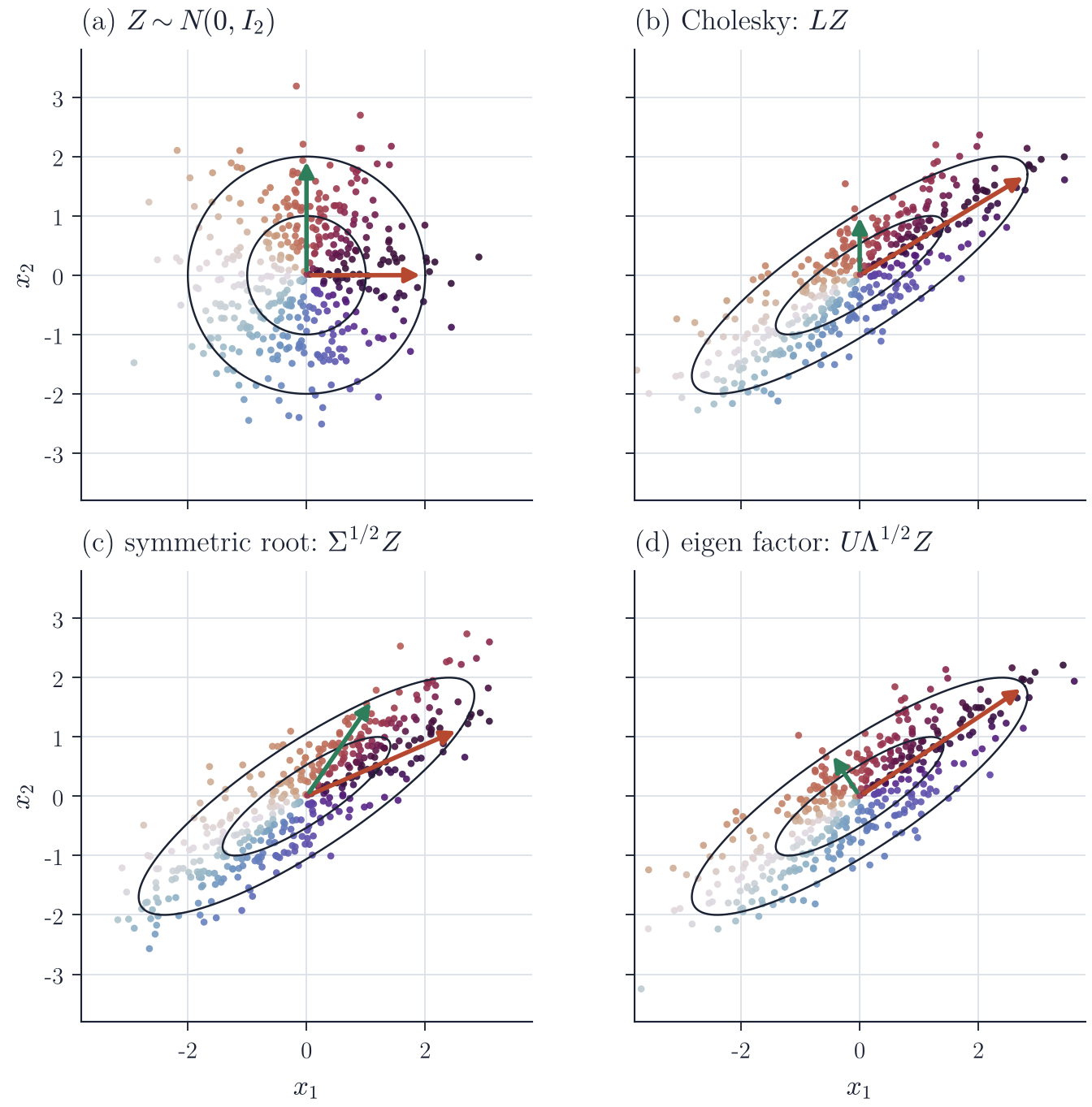
The same 400 standard normal draws mapped by three different square roots of one covariance matrix, giving identical elliptical clouds with differently arranged colours — Figure 1. (a) 400 draws of $Z \sim N(0, I_2)$, coloured by angle, with the circles of radius 1 and 2 and twice the basis vectors $e_1$ (red) and $e_2$ (green). (b)–(d) The same draws mapped by three factors of $\Sigma = \begin{pmatrix} 2 & 1.2 \\ 1.2 & 1 \end{pmatrix}$. The ellipses $\{x : x^\top\Sigma^{-1}x = r^2\}$ coincide; the images of $e_1$ and $e_2$ do not. The Cholesky factor keeps $Le_2$ on the $x_2$ axis, and the eigen factor sends $e_1$ and $e_2$ to the principal axes.

The eigen factor and the geometry. With $A = U\Lambda^{1/2}$,

\[X = \mu + \sum_{j=1}^p \sqrt{\lambda_j}\, Z_j\, u_j ,\]

a sum of independent contributions along orthogonal directions with standard deviations $\sqrt{\lambda_j}$. The density contours $\{x : (x - \mu)^\top\Sigma^{-1}(x-\mu) = c\}$ are ellipsoids with semi-axes $\sqrt{c\lambda_j}\, u_j$, and truncating the sum after $q$ terms gives the orthogonal projection of $X$ onto the $q$-dimensional affine subspace that approximates it best in mean square, which is the population form of principal component analysis.

The same representation handles a singular $\Sigma$ of rank $r < p$. Then $\lambda_{r+1} = \cdots = \lambda_p = 0$, so $X$ lies almost surely in the affine subspace $\mu + \mathrm{span}(u_1, \dots, u_r)$ and has no density with respect to Lebesgue measure on $\R^p$. With the pseudoinverse $\Sigma^+ = \sum_{j \le r} \lambda_j^{-1}u_ju_j^\top$,

\[(X - \mu)^\top \Sigma^+ (X - \mu) = \sum_{j=1}^r \frac{(\sqrt{\lambda_j} Z_j)^2}{\lambda_j} = \sum_{j=1}^r Z_j^2 \sim \chi^2_r ,\]

which is the version of the Mahalanobis distance that remains valid in the singular case. Numerically, the eigendecomposition is also the robust choice when a covariance matrix that should be positive semi-definite has small negative eigenvalues from rounding: they can be set to zero before forming the factor, whereas a Cholesky factorization would fail.

The Cholesky factor and sequential regression. The triangular structure of $L$ has a direct probabilistic meaning.

Proposition 3. Let $\Sigma \succ 0$, $\Sigma = LL^\top$ with $L$ lower triangular with positive diagonal, and $X = \mu + LZ$ with $Z \sim N_p(0, I_p)$. For each $j$, writing $X_{<j} = (X_1, \dots, X_{j-1})$,

\[\E[X_j \mid X_{<j}] = \mu_j + \sum_{i<j} L_{ji} Z_i, \qquad \Var(X_j \mid X_{<j}) = L_{jj}^2, \qquad Z_j = \frac{X_j - \E[X_j \mid X_{<j}]}{L_{jj}} .\]

In particular $\det \Sigma = \prod_{j=1}^p \Var(X_j \mid X_{<j})$.

Proof. Because $L$ is lower triangular, $X_{<j} = \mu_{<j} + L_{<j}Z_{<j}$, where $L_{<j}$ is the leading $(j-1) \times (j-1)$ block of $L$, which is invertible. Hence $X_{<j}$ and $Z_{<j}$ are bijective affine functions of each other and generate the same $\sigma$-field. In $X_j = \mu_j + \sum_{i<j}L_{ji}Z_i + L_{jj}Z_j$ the middle sum is a function of $Z_{<j}$ and $Z_j$ is independent of $Z_{<j}$ with mean zero and variance one. The conditional mean and variance follow, and the last identity is a rearrangement. Finally $\det\Sigma = (\det L)^2 = \prod_j L_{jj}^2$.

The standardized innovations $Z_j$ are what Gram–Schmidt orthogonalization of $X_1 - \mu_1, \dots, X_p - \mu_p$ produces in $L^2(\P)$, so the Cholesky factorization of a covariance matrix is Gram–Schmidt applied to random variables. The determinant identity is the prediction error decomposition used to evaluate Gaussian likelihoods of time series, and the conditional representation is the basis of the modified Cholesky decomposition used to parametrize covariance matrices through autoregressions. The price is dependence on the ordering: permuting the variables changes $L$ in ways that are not a simple permutation of its entries, so the Cholesky factor is natural only when the variables come in a meaningful order, such as time.

The symmetric root. $\Sigma^{1/2}$ is the only factor that is itself symmetric positive definite, and it commutes with $\Sigma$. It is the convenient choice in proofs, for instance in writing $\Sigma^{-1/2}(X - \mu) \sim N_p(0, I_p)$ without reference to a basis. Among all factors it is also the one closest to the identity. Every factor is $A = \Sigma^{1/2}Q$ with $Q$ orthogonal, and $\tr(\Sigma^{1/2}Q) = \sum_j \sqrt{\lambda_j}\, u_j^\top Q u_j \le \tr(\Sigma^{1/2})$ with equality only for $Q = I_p$. Since $\E\lVert AZ - Z\rVert^2 = \tr\Sigma - 2\tr A + p$, the map $z \mapsto \Sigma^{1/2}z$ moves points the least in mean square among all linear maps carrying $N_p(0, I_p)$ to $N_p(0, \Sigma)$; it is in fact the optimal transport map between the two laws. The same optimality reappears for whitening transformations, which apply the inverse of a factor to data.

Practical comparison

For sampling from a fixed $\Sigma \succ 0$, the Cholesky factor is the cheapest, about $p^3/3$ flops once and then $p^2$ per draw for the triangular product. The eigendecomposition costs a larger multiple of $p^3$ but tolerates singular and slightly indefinite matrices and gives the principal axes as a by-product. For log-densities, Cholesky gives $\log\det\Sigma = 2\sum_j \log L_{jj}$ and the quadratic form $\lVert L^{-1}(x - \mu)\rVert^2$ by one forward substitution. Whatever the factor, the generated sample has the same law, so the choice is about cost, numerical robustness and interpretation, and never about correctness.

Standard references are Anderson, An Introduction to Multivariate Statistical Analysis, for the distribution theory, and Golub and Van Loan, Matrix Computations, for the factorizations.