Stochastic EM for Gaussian mixtures

The note on EM for Gaussian mixtures derived an algorithm that increases the likelihood at every step and converges, under regularity conditions, to a stationary point. Two weaknesses remain. EM can be very slow when the current fit is near a saddle point or a poorly separated configuration, and which stationary point it reaches is fixed by the starting value. Stochastic EM (SEM), introduced by Celeux and Diebolt, changes one ingredient: instead of averaging the complete-data log-likelihood over the posterior of the latent labels, it samples the labels once and maximizes the resulting complete-data likelihood. Below, SEM is derived for Gaussian mixtures, the iteration is identified as a Markov chain, and the two algorithms are compared on a small example.

The E-step as a prediction

Let $x = (x_1, \dots, x_n)$ be the observed data and $Z = (Z_1, \dots, Z_n)$ the latent labels, and write $L_c(\Theta; z) = \log p(x, z; \Theta)$ for the complete-data log-likelihood. The E-step of EM computes

\[Q(\Theta \mid \Theta_t) = \E_{\Theta_t}\bigl[L_c(\Theta; Z) \mid x\bigr] = \sum_{z} L_c(\Theta; z)\, p(z \mid x; \Theta_t),\]

a finite sum because each $Z_i$ takes values in $\{1, \dots, K\}$. For each fixed $\Theta$ this is the conditional expectation of the unknown quantity $L_c(\Theta; Z)$ given the data, computed as if $\Theta_t$ were the true parameter. A conditional expectation is the best predictor in mean square: among all constants $c$,

\[Q(\Theta \mid \Theta_t) = \argmin_{c \in \R}\, \sum_{z}\bigl(L_c(\Theta; z) - c\bigr)^2 p(z \mid x; \Theta_t),\]

since the right-hand side is a quadratic in $c$ minimized at the posterior mean. EM thus maximizes the best available prediction of the complete-data log-likelihood. SEM maximizes a single random draw of it instead. If $Z^{(t)} \sim p(\cdot \mid x; \Theta_t)$, then $\E_{\Theta_t}[L_c(\Theta; Z^{(t)}) \mid x] = Q(\Theta \mid \Theta_t)$ for every fixed $\Theta$, so the random objective is unbiased for $Q$. Its maximizer, however, is not unbiased for the maximizer of $Q$, and this is the source of both the strengths and the defects of the method.

The algorithm

Given $\Theta_t$, one SEM iteration is:

S-step. Draw $Z^{(t)} = (Z_1^{(t)}, \dots, Z_n^{(t)})$ from $p(z \mid x; \Theta_t)$.
M-step. Set $\Theta_{t+1} = \argmax_\Theta L_c(\Theta; Z^{(t)})$, the complete-data maximum likelihood estimator for the imputed labels.

For a mixture of $K$ normal distributions $\mathcal{N}(\mu_k, \Sigma_k)$ with weights $\pi_k$, the labels are conditionally independent given the data, with

\[\P(Z_i = k \mid x_i; \Theta_t) = \gamma_{t,ik} = \frac{\pi_{t,k}\,\phi(x_i; \mu_{t,k}, \Sigma_{t,k})}{\sum_{j=1}^K \pi_{t,j}\,\phi(x_i; \mu_{t,j}, \Sigma_{t,j})},\]

so the S-step draws each $Z_i^{(t)}$ independently from the categorical distribution with probabilities $(\gamma_{t,i1}, \dots, \gamma_{t,iK})$. The responsibilities are the same as in EM; only their use differs.

With labels $z = Z^{(t)}$ fixed, write $I_k = \{i : z_i = k\}$ and $N_k = \lvert I_k \rvert$. The complete-data log-likelihood separates:

\[L_c(\Theta; z) = \sum_{k=1}^K N_k\log\pi_k + \sum_{k=1}^K\sum_{i \in I_k}\log\phi(x_i; \mu_k, \Sigma_k).\]

This is the function maximized in the M-step of EM with each responsibility $\gamma_{t,ik}$ replaced by the indicator $\mathbf 1\{z_i = k\}$. The proof given there therefore applies verbatim: if every $N_k \ge 1$ and every matrix $S_k = \sum_{i \in I_k}(x_i - \bar x_k)(x_i - \bar x_k)^\top$ is positive definite, the unique maximizer is

\[\pi_{t+1,k} = \frac{N_k}{n}, \qquad \mu_{t+1,k} = \bar x_k = \frac{1}{N_k}\sum_{i \in I_k} x_i, \qquad \Sigma_{t+1,k} = \frac{1}{N_k}\sum_{i \in I_k}(x_i - \bar x_k)(x_i - \bar x_k)^\top .\]

Each component is refitted to the points currently assigned to it, by their proportion, sample mean and sample covariance with divisor $N_k$. For the covariances, the stationarity condition in $\Sigma_k$ reads

\[-\frac{N_k}{2}\Sigma_k^{-1} + \frac12\Sigma_k^{-1}\Bigl(\sum_{i \in I_k}(x_i - \mu_k)(x_i - \mu_k)^\top\Bigr)\Sigma_k^{-1} = 0,\]

and the fact that the solution is a maximum, not merely a stationary point, follows from the eigenvalue argument in the earlier note.

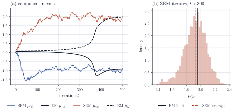
The hypotheses now have real content. Unlike the responsibilities in EM, which are all positive, the S-step can leave a component with too few points: $S_k$ is positive definite only if the points in $I_k$ affinely span $\R^d$, which requires $N_k \ge d + 1$. This happens with positive probability at every iteration, and some rule is needed. A simple one, used in Figure 1, is to redraw the labels until every component has at least $d + 1$ points that are not contained in an affine hyperplane; alternatives are to re-initialize the component or to drop it and continue with $K - 1$ components.

What SEM produces

Because $Z^{(t)}$ is drawn afresh at every step, $\Theta_{t+1}$ is random even given $\Theta_t$, and the sequence never settles at a point. Its structure is easiest to see through the labels. The M-step makes $\Theta_{t+1}$ a deterministic function of $Z^{(t)}$, and $Z^{(t+1)}$ is drawn from a distribution that depends only on $\Theta_{t+1}$. Hence, given the data, $(Z^{(t)})_{t \ge 0}$ is a time-homogeneous Markov chain on the finite set of admissible labellings. With the redrawing rule, every admissible labelling has positive probability of being drawn from any state, since all responsibilities are positive. A finite Markov chain with all transition probabilities positive is irreducible and aperiodic, so it has a unique stationary distribution $\varpi$ and its law converges to $\varpi$ from any start. Write $\Theta_{t+1} = M(Z^{(t)})$ for the M-step map. For every function $h$ of the parameter, the ergodic theorem for finite Markov chains gives

\[\frac1T\sum_{t=1}^T h(\Theta_t) \xrightarrow{\text{a.s.}} \sum_{z} h\bigl(M(z)\bigr)\,\varpi(z), \qquad T \to \infty,\]

for the fixed data set; the randomness here is that of the algorithm, not of the data.

The function $h$ must be chosen with care. Permuting the labels of $z$ permutes the components of $M(z)$, and the transition probabilities are unchanged when the labels of both the current and the next state are permuted in the same way. Since $\varpi$ is unique, it is therefore invariant under relabelling, and the stationary mean of $\Theta_t$ itself has all components equal: averaging raw iterates is meaningless in the long run. One averages instead a label-invariant summary, for instance the parameters with components ordered by their means, as in Figure 1. When the components are well separated, label switches are so rare that a run of practical length stays near a single labelling, but the ordering removes the problem altogether.

The Markov chain structure has two further consequences. First, SEM forgets its starting value, which EM never does. Second, SEM has no monotonicity: the likelihood fluctuates along the chain, and convergence diagnostics for EM, such as a small increase of $\ell(\Theta_t)$, are meaningless. The standard outputs are the average of the ordered iterates after a burn-in period, or the iterate with the largest likelihood, often followed by a few EM steps to reach a nearby stationary point. When the components are well identified and $n$ is large, the iterates fluctuate, up to relabelling, at distance of order $n^{-1/2}$ around a point near the maximum likelihood estimate; Nielsen (2000) gives conditions under which the SEM estimator is consistent and asymptotically normal, with an asymptotic variance larger than that of the maximum likelihood estimator. For finite $n$, the stationary mean generally differs from the maximum likelihood estimate.

An example

Figure 1 compares EM and SEM on $n = 400$ observations from the univariate mixture $0.65\,\mathcal{N}(-1, 1.2^2) + 0.35\,\mathcal{N}(2, 0.8^2)$, fitting two components with unequal variances. Both algorithms start from equal weights, variances $3$ and means $\pm 0.01$, almost on top of each other.

The start matters for EM. With equal weights and variances and equal means, all responsibilities equal $1/2$, and the M-step returns two identical components with the sample mean and variance: the symmetric configuration is a fixed point of EM. It is unstable, so a start at distance $\delta$ from it escapes, but only at a geometric rate, and the number of iterations needed grows like $\log(1/\delta)$. In this example EM needs about 430 iterations to come within $0.1$ of its limit; with means $\pm 0.2$ it needs about 140. SEM is unaffected by the near-symmetry: the random labels break the tie in the first few iterations. In fifty independent runs from the same start, SEM first came within $0.15$ of the EM limit after a median of about 80 iterations, with a range of roughly 30 to 260.

Panel (b) shows the price. After burn-in, the larger mean fluctuates with a standard deviation of about $0.15$, roughly twice the standard error $0.8/\sqrt{140} \approx 0.07$ that the mean of the second component would have if the labels were known, and its average $1.92$ differs slightly from the EM limit $1.96$. SEM is therefore best used to explore and to escape, and EM to finish.

Left: trajectories of the two component means under EM, which stay near zero for about 350 iterations before separating, and under SEM, which separate within about 50 iterations and then fluctuate. Right: histogram of SEM iterates of the larger mean with the EM limit and the SEM average marked. — Figure 1. Two-component univariate mixture, $n = 400$, started from means $\pm 0.01$. (a) The ordered means $\mu_{(1)} \le \mu_{(2)}$ along EM (black) and along one SEM run (colour). (b) SEM iterates of $\mu_{(2)}$ for $300 < t \le 3000$, with the EM limit (solid) and the SEM average (dashed). Components are ordered by their means at each iteration, which removes the label switching that SEM is free to perform.

Summary of the iteration

For $t = 0, 1, \dots, T - 1$:

compute the responsibilities $\gamma_{t,ik}$ for all $i$ and $k$, on the log scale;
draw $Z_i^{(t)} \sim \mathrm{Categorical}(\gamma_{t,i1}, \dots, \gamma_{t,iK})$ independently over $i$, and redraw if some component receives fewer than $d + 1$ points;
set $N_k = \lvert\{i : Z_i^{(t)} = k\}\rvert$, $\pi_{t+1,k} = N_k/n$, and let $\mu_{t+1,k}$ and $\Sigma_{t+1,k}$ be the sample mean and covariance (divisor $N_k$) of the points assigned to component $k$.

Report the average of $\Theta_t$ over $t > t_0$ after ordering the components by a fixed rule, or use the best iterate as the starting value for EM. The cost per iteration is that of EM, since the responsibilities must still be computed.

Remarks

SEM sits between two other modifications of EM. Monte Carlo EM (Wei and Tanner, 1990) approximates $Q(\Theta \mid \Theta_t)$ by an average over $m$ draws of the labels; SEM is the case $m = 1$, and letting $m$ grow with $t$ recovers the behaviour of EM. The stochastic approximation EM algorithm (Delyon, Lavielle and Moulines, 1999) averages the simulated complete-data objectives over iterations with decreasing weights, which, under regularity conditions, turns the fluctuating chain into a sequence that converges almost surely to a stationary point of the likelihood. In the other direction, classification EM (Celeux and Govaert, 1992) replaces sampling by assigning each point to its most probable component; for spherical components with equal weights and a common variance this is the $k$-means algorithm, and it estimates the parameters with a bias that does not vanish as $n \to \infty$.

The original reference is Celeux and Diebolt, “The SEM algorithm: a probabilistic teacher algorithm derived from the EM algorithm for the mixture problem” (1985). Asymptotic theory is in Nielsen, “The stochastic EM algorithm: estimation and asymptotic results” (Bernoulli, 2000), and McLachlan and Krishnan, The EM Algorithm and Extensions, surveys the stochastic variants.