Boole's inequality and the union bound
Boole’s inequality bounds the probability of a union by the sum of the individual probabilities. It requires nothing about the dependence between the events, which is why it appears in so many arguments: whenever a statement must hold simultaneously for many indices, one bounds the probability that it fails for each index and adds. The price of ignoring dependence is that the bound can be far from sharp, and part of this note is about when it is sharp.
Throughout, \((\Omega, \mathcal F, \P)\) is a probability space and all sets \(A_i\) belong to \(\mathcal F\).
Theorem 1 (Boole’s inequality). For events \(A_1, \dots, A_n\),
\[\P\Bigl(\bigcup_{i=1}^n A_i\Bigr) \le \sum_{i=1}^n \P(A_i),\]and for a sequence of events \(A_1, A_2, \dots\),
\[\P\Bigl(\bigcup_{i=1}^\infty A_i\Bigr) \le \sum_{i=1}^\infty \P(A_i).\]Equality holds, in either case, if and only if \(\P(A_i \cap A_j) = 0\) for all \(i \ne j\).
The countable statement is called countable subadditivity of \(\P\). It is the nontrivial one: the finite statement follows from finite additivity alone, while the countable one needs countable additivity.
First proof: induction and continuity
For two events, \(A_1 \cup A_2\) is the disjoint union of \(A_1\) and \(A_2 \setminus A_1\), and \(A_2\) is the disjoint union of \(A_2 \setminus A_1\) and \(A_1 \cap A_2\). Finite additivity therefore gives
\[\P(A_1 \cup A_2) = \P(A_1) + \P(A_2) - \P(A_1 \cap A_2) \le \P(A_1) + \P(A_2).\]Suppose the finite inequality holds for \(n\) events and write \(B_n = \bigcup_{i=1}^n A_i\). Applying the two-event case to \(B_n\) and \(A_{n+1}\) and then the induction hypothesis,
\[\P(B_{n+1}) = \P(B_n) + \P(A_{n+1}) - \P(B_n \cap A_{n+1}) \le \sum_{i=1}^{n} \P(A_i) + \P(A_{n+1}).\]Induction proves the finite statement for every \(n\), but it does not reach the countable one by itself: knowing the inequality for each finite \(n\) says nothing yet about the infinite union. The missing step is continuity from below. The sets \(B_n\) increase to \(B = \bigcup_{i=1}^\infty A_i\), so \(\P(B_n) \to \P(B)\), and letting \(n \to \infty\) in \(\P(B_n) \le \sum_{i=1}^n \P(A_i) \le \sum_{i=1}^\infty \P(A_i)\) gives the countable statement. Continuity from below is itself a consequence of countable additivity, applied to the disjoint pieces \(B_1, B_2 \setminus B_1, B_3 \setminus B_2, \dots\).
Second proof: disjoint pieces
The second proof uses countable additivity directly. Define
\[C_1 = A_1, \qquad C_i = A_i \setminus \bigcup_{j=1}^{i-1} A_j \quad (i \ge 2).\]Each \(C_i\) is an event, \(C_i \subseteq A_i\), and the \(C_i\) are pairwise disjoint: if \(j < i\), then \(C_j \subseteq A_j\) while \(C_i\) excludes \(A_j\). They have the same union as the \(A_i\), because a point of \(\bigcup_i A_i\) belongs to \(C_k\) for the smallest \(k\) with that point in \(A_k\). Hence, by countable additivity and monotonicity,
\[\P\Bigl(\bigcup_{i=1}^\infty A_i\Bigr) = \P\Bigl(\bigcup_{i=1}^\infty C_i\Bigr) = \sum_{i=1}^\infty \P(C_i) \le \sum_{i=1}^\infty \P(A_i).\]The finite case is the special case \(A_i = \emptyset\) for \(i > n\). No monotonicity of the sequence \(A_i\) is needed.
Third proof: indicators
The cleanest proof works pointwise. Every \(\omega\) in the union lies in at least one \(A_i\), so
\[\mathbf 1_{\bigcup_i A_i}(\omega) \le \sum_{i=1}^\infty \mathbf 1_{A_i}(\omega) \qquad \text{for all } \omega \in \Omega ,\]where the right-hand side is the number of events containing \(\omega\), possibly \(+\infty\). Taking expectations and exchanging expectation and sum, which is allowed for nonnegative terms by the monotone convergence theorem,
\[\P\Bigl(\bigcup_{i} A_i\Bigr) \le \E \sum_{i} \mathbf 1_{A_i} = \sum_{i} \P(A_i).\]This proof also gives the equality statement of Theorem 1. Let \(D = \sum_i \mathbf 1_{A_i} - \mathbf 1_{\bigcup_i A_i}\), a nonnegative random variable that counts, for each \(\omega\) in the union, the events containing \(\omega\) beyond the first. If \(\sum_i \P(A_i) < \infty\), then \(\E D = \sum_i \P(A_i) - \P(\bigcup_i A_i)\), and this is zero if and only if \(D = 0\) almost surely, that is, if and only if almost no \(\omega\) belongs to two of the events. Since \(\{D \ge 1\} = \bigcup_{i < j} (A_i \cap A_j)\) is a countable union, this happens exactly when \(\P(A_i \cap A_j) = 0\) for every pair \(i \ne j\). If \(\sum_i \P(A_i) = \infty\), the inequality is strict because the left side is at most one, and the intersections cannot all be null, since otherwise the same computation would give \(\sum_i \P(A_i) = \P(\bigcup_i A_i) \le 1\).
The size of \(D\) measures the slack. When the events overlap heavily, \(\E D\) is large and the bound is poor; the extreme case \(A_1 = A_2 = \dots = A_m\) overestimates \(\P(A_1)\) by a factor of \(m\).
A lower bound
The pointwise argument extends to a lower bound with a correction for pairwise overlaps.
Proposition 2 (Bonferroni). For events \(A_1, \dots, A_n\),
\[\sum_{i=1}^n \P(A_i) - \sum_{1 \le i < j \le n} \P(A_i \cap A_j) \le \P\Bigl(\bigcup_{i=1}^n A_i\Bigr) \le \sum_{i=1}^n \P(A_i).\]Proof. Only the left inequality is new. Fix \(\omega\) and let \(k\) be the number of indices \(i\) with \(\omega \in A_i\). Evaluated at \(\omega\), the random variable \(\sum_i \mathbf 1_{A_i} - \sum_{i<j} \mathbf 1_{A_i \cap A_j}\) equals \(k - \binom k2 = k(3-k)/2\). For \(k = 0\) this is \(0 = \mathbf 1_{\bigcup_i A_i}(\omega)\). For integers \(k \ge 1\) it is at most \(1 = \mathbf 1_{\bigcup_i A_i}(\omega)\), since \(k(3-k)/2 \le 1\) is equivalent to \((k-1)(k-2) \ge 0\). Taking expectations of the resulting pointwise inequality gives the claim.
These are the first two of the Bonferroni inequalities, which are the partial sums of the inclusion–exclusion formula, alternately bounding \(\P(\bigcup_i A_i)\) from above and below. If \(\sum_{i<j} \P(A_i \cap A_j)\) is small compared with \(\sum_i \P(A_i)\), the two bounds of Proposition 2 nearly agree and Boole’s inequality is close to an equality.
Two uses
Multiple testing. Suppose \(m\) null hypotheses are tested with p-values \(p_1, \dots, p_m\), and that each p-value is valid under its null: \(\P(p_i \le u) \le u\) for \(u \in [0, 1]\) whenever hypothesis \(i\) is true. The Bonferroni procedure rejects hypothesis \(i\) when \(p_i \le \alpha/m\). If \(I_0\) is the set of true nulls, with \(m_0\) elements, the probability of at least one false rejection is
\[\P\Bigl(\bigcup_{i \in I_0} \{p_i \le \alpha/m\}\Bigr) \le \sum_{i \in I_0} \P(p_i \le \alpha/m) \le \frac{m_0\, \alpha}{m} \le \alpha .\]The family-wise error rate is controlled under arbitrary dependence between the tests, which is the procedure’s main virtue; the price is conservativeness when the tests are strongly dependent.
Maxima of Gaussian variables. Let \(Z_1, \dots, Z_m\) be standard normal, with any joint distribution. For \(t \ge 0\) and \(\lambda > 0\), Markov’s inequality applied to \(e^{\lambda Z_1}\) gives \(\P(Z_1 > t) \le e^{-\lambda t}\, \E e^{\lambda Z_1} = e^{-\lambda t + \lambda^2/2}\), and the choice \(\lambda = t\) gives \(\P(Z_1 > t) \le e^{-t^2/2}\). The union bound over the \(2m\) events \(\{Z_i > t\}\) and \(\{-Z_i > t\}\) then gives
\[\P\Bigl(\max_{i \le m} \abs{Z_i} > t\Bigr) \le 2m\, e^{-t^2/2}.\]Setting \(t = \sqrt{2 \log(2m/\delta)}\), with probability at least \(1 - \delta\) all \(m\) variables are bounded in absolute value by \(\sqrt{2\log(2m/\delta)}\). The logarithmic dependence on \(m\) is what makes union bounds useful in high-dimensional statistics: a bound for one coordinate costs only a \(\sqrt{\log m}\) factor to extend to \(m\) coordinates.
The figure compares the union bound \(m\bar\Phi(t)\), where \(\bar\Phi = 1 - \Phi\) is the standard normal tail, with the exact probability \(\P(\max_i Z_i > t)\) when the \(Z_i\) are equicorrelated, \(Z_i = \sqrt\rho\, W + \sqrt{1-\rho}\, E_i\) with \(W, E_1, \dots, E_m\) i.i.d. standard normal.
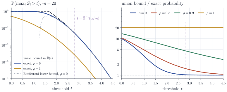
Two features stand out. For independent variables the bound is almost exact in the region that matters for testing: at the Bonferroni threshold \(t \approx 2.81\) the exact probability is \(0.0488\), against the nominal \(0.05\). This agrees with Proposition 2, since the correction term \(\binom m2 \bar\Phi(t)^2\) is of smaller order than \(m\bar\Phi(t)\) when \(m\bar\Phi(t)\) is small. Under strong dependence the bound is loose: at the same threshold the exact probabilities are about \(0.033\), \(0.011\) and \(0.0025\) for \(\rho = 0.5\), \(0.9\) and \(1\), and in the last case the bound is off by the full factor \(m\). For every fixed \(\rho < 1\) the ratio still tends to one as \(t \to \infty\), because \(\P(Z_i > t, Z_j > t)/\P(Z_i > t) \to 0\) for a bivariate normal pair with correlation less than one; but the convergence is slow when \(\rho\) is close to one.
Remarks
The union bound is also the basic tool for uniform bounds over finite families, for instance in learning theory, where a deviation inequality for a single classifier is extended to a finite class \(\mathcal H\) at the cost of a factor \(\lvert \mathcal H \rvert\) in probability, that is, an additive \(\log \lvert \mathcal H \rvert\) in the exponent. For infinite classes, chaining and VC arguments refine exactly this step by grouping events that overlap heavily.
Countable subadditivity holds for every measure, not only for probability measures, by the same disjointification argument. A standard reference is Billingsley, Probability and Measure.