Bessel's correction: why the sample variance divides by n − 1
Every introductory course defines the sample variance with the divisor \(n-1\) rather than \(n\), and the usual justification is that the result is unbiased. The reason is simple once seen: deviations are measured from the sample mean \(\bar X\), which is itself fitted to the data and therefore sits closer to the observations than the population mean \(\mu\) does. Below are a direct proof, two other proofs that explain the factor \(n-1\) from different angles, and the less often mentioned fact that unbiasedness and small mean squared error point to different divisors.
Setting
Let \(X_1, \dots, X_n\) be random variables with a common mean \(\mu = \E X_i\) and a common finite variance \(\sigma^2 = \Var(X_i)\), and assume they are pairwise uncorrelated. An i.i.d. sample with \(\E X_1^2 < \infty\) is the main example, but nothing more than these second-moment conditions is needed for unbiasedness. Assume \(n \ge 2\) and write
\[\bar X = \frac1n \sum_{i=1}^n X_i, \qquad \mathrm{SS} = \sum_{i=1}^n (X_i - \bar X)^2, \qquad S^2 = \frac{\mathrm{SS}}{n-1}, \qquad \hat\sigma^2 = \frac{\mathrm{SS}}{n}.\]An estimator \(T\) of a quantity \(\tau\) is unbiased if \(\E T = \tau\) for every distribution in the model under consideration; its bias is \(\E T - \tau\). Here the model is the set of all distributions satisfying the conditions above, so unbiasedness of \(S^2\) means \(\E S^2 = \sigma^2\) whatever the values of \(\mu\) and \(\sigma^2\).
Proposition 1. Under the conditions above, \(\E\,\mathrm{SS} = (n-1)\sigma^2\). Consequently \(\E S^2 = \sigma^2\) and \(\E \hat\sigma^2 = \bigl(1 - \tfrac1n\bigr)\sigma^2\).
A direct computation
Proof of Proposition 1. Expanding the square and using \(\sum_i X_i = n\bar X\),
\[\mathrm{SS} = \sum_{i=1}^n X_i^2 - 2\bar X \sum_{i=1}^n X_i + n\bar X^2 = \sum_{i=1}^n X_i^2 - n\bar X^2 .\]For any random variable \(Y\) with finite variance, \(\E Y^2 = \Var(Y) + (\E Y)^2\). Applied to \(X_i\) this gives \(\E X_i^2 = \sigma^2 + \mu^2\). Applied to \(\bar X\), whose mean is \(\mu\) and whose variance is
\[\Var(\bar X) = \frac{1}{n^2} \sum_{i=1}^n \sum_{j=1}^n \Cov(X_i, X_j) = \frac{1}{n^2} \sum_{i=1}^n \Var(X_i) = \frac{\sigma^2}{n}\]because the off-diagonal covariances vanish, it gives \(\E \bar X^2 = \sigma^2/n + \mu^2\). Hence
\[\E\,\mathrm{SS} = n(\sigma^2 + \mu^2) - n\Bigl(\frac{\sigma^2}{n} + \mu^2\Bigr) = (n-1)\sigma^2 .\]Dividing by \(n-1\) and by \(n\) gives the two remaining claims.
The computation shows where the missing \(\sigma^2\) goes. Had we centred at \(\mu\), the expected sum of squares would be \(\sum_i \E(X_i - \mu)^2 = n\sigma^2\). The identity
\[\sum_{i=1}^n (X_i - \mu)^2 = \mathrm{SS} + n(\bar X - \mu)^2\](expand \(X_i - \mu = (X_i - \bar X) + (\bar X - \mu)\); the cross term vanishes because \(\sum_i (X_i - \bar X) = 0\)) splits \(n\sigma^2\) into \(\E\,\mathrm{SS}\) and \(n\E(\bar X - \mu)^2 = n \Var(\bar X) = \sigma^2\). Because \(\bar X\) minimizes \(c \mapsto \sum_i (X_i - c)^2\), centring at the sample mean always gives a smaller sum of squares than centring at \(\mu\), and on average the difference is exactly one \(\sigma^2\).
Two other proofs
Pairwise differences. Summing \((X_i - X_j)^2\) over all ordered pairs and expanding,
\[\sum_{i=1}^n \sum_{j=1}^n (X_i - X_j)^2 = 2n \sum_{i=1}^n X_i^2 - 2\Bigl(\sum_{i=1}^n X_i\Bigr)^2 = 2n\,\mathrm{SS},\]so that
\[S^2 = \frac{1}{n(n-1)} \sum_{i < j} (X_i - X_j)^2 .\]The sample variance is the average of \(\tfrac12 (X_i - X_j)^2\) over the \(\binom n2\) unordered pairs. For \(i \ne j\), \(\E (X_i - X_j)^2 = \Var(X_i - X_j) = 2\sigma^2\) by uncorrelatedness, which proves \(\E S^2 = \sigma^2\) again. This representation makes the divisor transparent: \(S^2\) averages over pairs of distinct observations, and there are \(n(n-1)/2\) of them. In the i.i.d. case it also shows that \(S^2\) is a U-statistic with kernel \(h(x, y) = (x-y)^2/2\).
Projection. Write \(X = (X_1, \dots, X_n)^\top\), \(\mathbf 1 = (1, \dots, 1)^\top\), and \(P = I_n - n^{-1}\mathbf 1 \mathbf 1^\top\). The matrix \(P\) is the orthogonal projection onto the \((n-1)\)-dimensional subspace \(\{v : \mathbf 1^\top v = 0\}\), the vector of residuals is \(PX\), and \(\mathrm{SS} = \norm{PX}^2 = X^\top P X\) since \(P\) is symmetric and idempotent. Under our assumptions \(\E X = \mu \mathbf 1\) and \(\Cov(X) = \sigma^2 I_n\), and for a fixed matrix \(A\) the identity \(\E X^\top A X = \tr\bigl(A \Cov(X)\bigr) + (\E X)^\top A\, \E X\) holds. Since \(P\mathbf 1 = 0\),
\[\E\,\mathrm{SS} = \sigma^2 \tr(P) + \mu^2\, \mathbf 1^\top P \mathbf 1 = \sigma^2 (n-1).\]Here \(n-1\) appears as the trace, equivalently the rank, of the residual projection. This is the sense of the phrase “one degree of freedom is spent on estimating the mean”, and the same calculation gives the divisor \(n - p\) for the residual sum of squares in a linear model with \(p\) linearly independent regressors, where \(P\) is replaced by the projection onto the orthogonal complement of the column space of the design matrix.
Unbiased is not the same as accurate
Unbiasedness is one criterion among several, and it is not preserved by nonlinear maps. Since the square root is strictly concave, Jensen’s inequality gives \(\E S \le \sqrt{\E S^2} = \sigma\), with strict inequality unless \(S\) is almost surely constant: the sample standard deviation is biased downward even though \(S^2\) is unbiased.
A second criterion is the mean squared error. Consider the family \(\mathrm{SS}/d\) for \(d > 0\). In addition to the previous assumptions, let the \(X_i\) be i.i.d. with \(\E X_1^4 < \infty\), and write \(\kappa = \E(X_1 - \mu)^4 / \sigma^4\) for the kurtosis, assuming \(\sigma > 0\). The pairwise representation gives the variance of \(S^2\) with little effort. Write \(h_{ij} = \tfrac12 (X_i - X_j)^2\), so that \(S^2\) is the average of \(h_{ij}\) over the \(N = \binom n2\) pairs and \(\Var(S^2) = N^{-2} \sum \Cov(h_{ij}, h_{kl})\), the sum running over all ordered couples of pairs. Couples of disjoint pairs are independent and contribute nothing. For a couple sharing exactly one index, say \(h_{12}\) and \(h_{13}\), conditioning on \(X_1\) and using \(\E[h_{12} \mid X_1] = \tfrac12\{(X_1 - \mu)^2 + \sigma^2\}\) gives \(\Cov(h_{12}, h_{13}) = \tfrac14 \Var\{(X_1-\mu)^2\} = \tfrac14 (\kappa - 1)\sigma^4\). For a couple of identical pairs, \(\Var(h_{12}) = \tfrac14 \E(X_1 - X_2)^4 - \sigma^4 = \tfrac12 (\kappa + 1)\sigma^4\), because \(\E(X_1 - X_2)^4 = 2\E(X_1-\mu)^4 + 6\sigma^4\) (the terms with an odd power of a centred variable vanish). There are \(N \cdot 2(n-2)\) couples of the first kind and \(N\) of the second, so
\[\Var(S^2) = \frac{2(n-2)\cdot\tfrac14(\kappa-1) + \tfrac12(\kappa+1)}{N}\,\sigma^4 = \sigma^4 \Bigl(\frac{\kappa}{n} - \frac{n-3}{n(n-1)}\Bigr).\]For normal data, \(\kappa = 3\) and this reduces to \(2\sigma^4/(n-1)\), which agrees with \(\mathrm{SS}/\sigma^2 \sim \chi^2_{n-1}\). With \(\E\,\mathrm{SS} = (n-1)\sigma^2\) and \(\E\,\mathrm{SS}^2 = (n-1)^2 \bigl(\Var(S^2) + \sigma^4\bigr)\), the mean squared error
\[\E\Bigl(\frac{\mathrm{SS}}{d} - \sigma^2\Bigr)^2 = \frac{\E\,\mathrm{SS}^2}{d^2} - \frac{2\sigma^2\,\E\,\mathrm{SS}}{d} + \sigma^4\]is a convex function of \(1/d\), minimized at \(1/d^\ast = \sigma^2\, \E\,\mathrm{SS} / \E\,\mathrm{SS}^2\). Substituting and simplifying,
\[d^\ast = n + 1 + \frac{(n-1)(\kappa - 3)}{n}.\]For normal data the best divisor is \(n+1\), not \(n-1\): dividing by \(n+1\) shrinks \(S^2\) by the factor \((n-1)/(n+1)\), and the bias this introduces is more than offset by the reduction in variance. For heavy-tailed data, where \(\kappa > 3\), the optimal divisor is larger still. For light-tailed data it is smaller; for symmetric \(\pm 1\) variables, where \(\kappa = 1\), one gets \(d^\ast = n - 1 + 2/n\), so the unbiased divisor is nearly optimal while \(n+1\) is a poor choice. Since \(\kappa\) is unknown in practice, \(d^\ast\) is not an estimator, but the comparison shows that no single divisor is best in mean squared error across distributions.
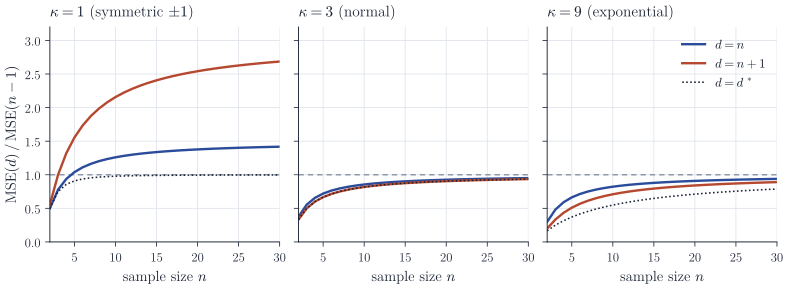
When \(\kappa > 1\) these differences are of lower order. The variance of \(S^2\) is \(\sigma^4(\kappa - 1)/n + O(n^{-2})\), while for a divisor \(d = n + c\) with \(c\) fixed the squared bias \(\{(c+1)\sigma^2/(n+c)\}^2\) and the change in variance are \(O(n^{-2})\); every mean squared error has the same leading term \(\sigma^4(\kappa - 1)/n\), and the ratios in Figure 1 tend to \(1\). The case \(\kappa = 1\) is degenerate: \((X_1 - \mu)^2\) is then almost surely constant, \(\Var(S^2) = 2\sigma^4/\{n(n-1)\}\) is itself of order \(n^{-2}\), and the squared bias is of the same order, so the ratios converge to \(3/2\) for \(d = n\) and to \(3\) for \(d = n + 1\), as the left panel shows. Apart from this case, the choice of divisor matters for small samples and for exact finite-sample statements, such as the \(t\) and \(F\) distributions, which are built on \(S^2\); it does not affect first-order asymptotics.
Remarks
The unbiasedness argument uses only first and second moments and uncorrelatedness, so it applies without change to, for example, exchangeable sequences with zero correlation. Under correlation it fails: if \(\Cov(X_i, X_j) = \rho\sigma^2\) for all \(i \ne j\), the projection argument gives \(\E\,\mathrm{SS} = \sigma^2 \tr\bigl(P\{(1-\rho)I_n + \rho\mathbf 1\mathbf 1^\top\}\bigr) = (n-1)(1-\rho)\sigma^2\), and no fixed divisor is unbiased for every \(\rho\). For time series the same effect is the reason that naive variance estimates are too small under positive autocorrelation.
For the variance computation and the normal-theory results, see Casella and Berger, Statistical Inference; for U-statistics, Serfling, Approximation Theorems of Mathematical Statistics.